Classification with Logistic Regression#
Since estimating posterior probabilities for some specific combination of characteristics is likely infeasible without a truly massive dataset, we need another way.
Logistic regression assumes that there is a mathematical relationship that gives the posterior probability based on a weighted sum of an individual’s characteristics. The goal from the data is thus not to estimate probabilities per se, but to estimate the correct set of weights.
This course will utilize logistic regression only for two-class classification (Yes vs. No).
There are extensions to logistic regression that handle multiple classes (see the \(VGAM\) package and read about multinomial logistic regression), but these days logistic regression is rarely the place to be in business analytics anyway, so the oversight is understandable.
Note: if \(p\) is the posterior probability output from the logistic regression model for the level of interest, the posterior probability of the other class is just \(1-p\).
For the sake of convenience and brevity, we will refer to posterior probabilities for the remainder of the discussion on logistic regression (and most other models) as just “probabilities”, i.e., dropping the word “posterior”.
Note
The probabilities output by the data mining algorithms we will discuss: logistic regression, partition models, neural networks, etc., are posterior probabilities (they are taking into account the characteristics of individuals).
When the classification model outputs a probability, the result will be between 0 and 1. You’ll likely be interested in actually making a prediction as to which class the individual belongs. How do we make the classification? By convention:
If \(p \ge 0.5\), classify the individual as having the class of interest (i.e., the one that comes last alphabetically).
If \(p < 0.5\), classify the individual as NOT having the class of interest (i.e., the one that comes first alphabetically).
Shortcut: calculate \(p\) (probability of class of interest) and \(1-p\) (probability of other class). Classify the individual by assigning whichever class has the higher probability.
Simple Logistic Regression model#
Simple logistic regression (predicting the probability from a single characteristic, i.e., one predictor variable \(x\)) relates \(p\) to \(x\) via the logit function (a transformation of \(p\))
Solving this equation for \(p\), our model for how \(p\) and \(x\) is related becomes:
Note
Note: logistic regression assumes that the relationship between \(p\) and \(x\) is nonlinear and well-described by the shape of the logistic curve.
Multiple Logistic Regression Model#
Often we want to predict the class of interest based on a variety of characteristics \(x_1\), \(x_2\), \(\ldots\), \(x_k\). The simple logistic regression model extends easily to incorporate more variables.
Solving this equation for \(p\), we can also write our model as:
Thus, multiple logistic regression predicts \(p\) from a weighted sum of predictors variables. Surprisingly, with the right choice of predictors, the model can be quite flexible and can capture a lot of relationships that simple logistic regression cannot.
Model: the Logistic Curve#
The equation \(p = \ldots\) is the equation for a “logistic” curve (which is why this is called logistic regression). This curve has a characteristic S shape which either starts out near 0 and curves up towards 1 or starts out near 1 and curves down to 0.
Note: the logistic model assumes that \(p\) is either always increasing with \(x\) or always decreasing.
par(mfrow=c(1,2))
curve( exp(-10+3*x)/(1+exp(-10+3*x)),from=1,to=6,xlab="x",ylab="p")
curve( exp(10-3*x)/(1+exp(10-3*x)),from=0,to=8,xlab="x",ylab="p")

Not always an appropriate model#
A linear regression does not provide a reasonable reflection of reality when the relationship between \(y\) and \(x\) is nonlinear. Similarly, a logistic regression does not provide a reasonable reflection of reality when the relationship between \(p\) and \(x\) is not well-described by a logistic curve.
The logistic curve often provides a decent approximation to how \(p\) changes (just as a straight line is often a decent approximation to how \(y\) varies with \(x\)) and is better than using no model at all, but stay vigilant.
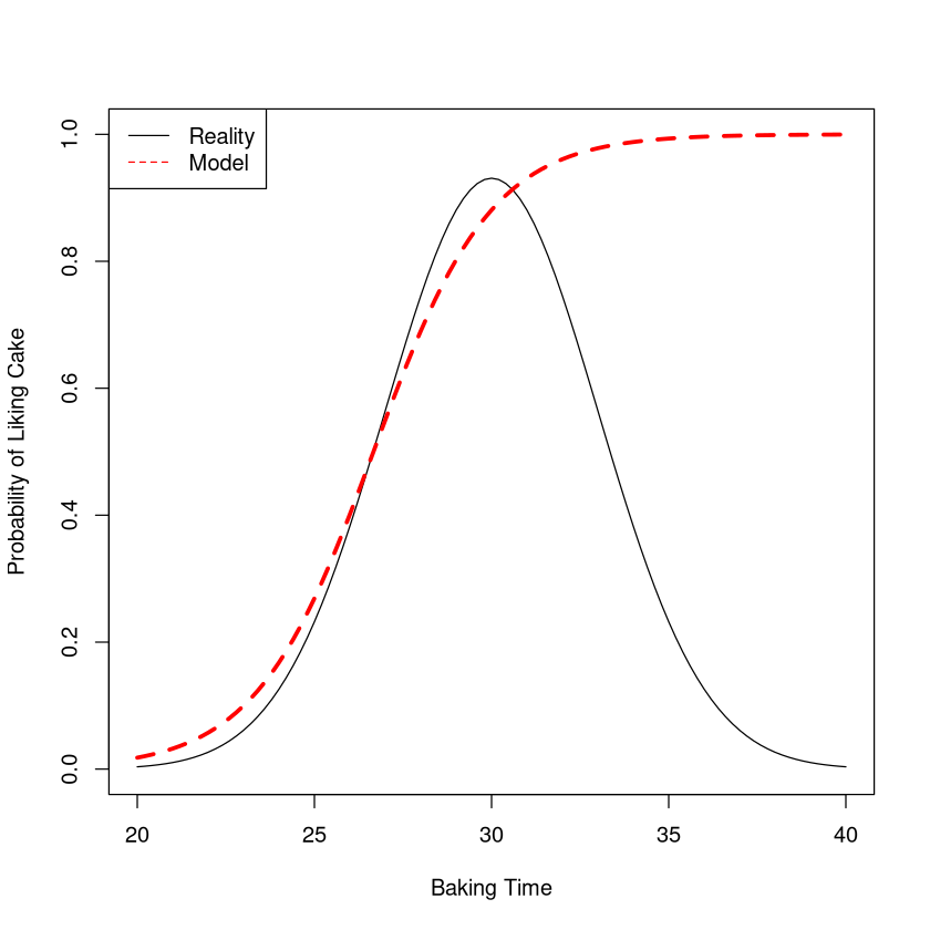
Imagine baking a cake and seeing if people like it. A simple logistic regression model would not be appropriate for studying how the probability of liking the cake varies with the baking time. For small baking times people won’t like it because it is undercooked. For large baking times people won’t like it because it is burned!
Logistic curve is NOT always a reasonable model#
The probability of liking a cake versus the baking time is definitely NOT well described by a logistic curve (red line), so a logistic regression would not be useful here in describing the relationship.
curve(7*dnorm(x,30,3),from=20,to=40,xlab="Baking Time",ylab="Probability of Liking Cake",ylim=c(0,1))
curve(1- exp(16-.6*x)/(1+exp(16-.6*x)),xlab="x",ylab="p",add=TRUE,col="red",lty=2,lwd=3)
legend("topleft",c("Reality","Model"),col=c("black","red"),lty=1:2)
Aside: flexibility of model when clever#
However, much like linear regression can be used to model nonlinear relationships (by using \(x^2\), \(x^3\), etc., as predictors), logistic regression can sometimes be used to model more sophisticated relationships. For example imagine using the model:
curve( exp(-45+3.1*x-0.05*x^2)/(1 + exp(-45+3.1*x-0.05*x^2)),from=0,to=60,xlab="Baking Time",ylab="Probability of Liking Cake",ylim=c(0,1))

This curve looks reasonable. However, how to know I should add \(x^2\) as a predictor?
In general, multiple logistic regression can model a variety of “shapes”, but it often requires deep insight to do so. With many data mining datasets having hundreds of variables, it’s typically not possible to stumble upon the “right” transformations.
When is simple logistic regression an OK model?#
A simple logistic regression model (predicting \(p\) from a single predictor variable \(x\)) may provide a reasonable reflection of reality if:
when we compare two individuals, the one with the larger value of \(x\) should always have a larger value of \(p\) (or always have a smaller value of \(p\)), irregardless of the \(x\)’s under consideration.
The above condition just means that the curve describing the probability is always rising (or always falling).
Although the logistic curve has the property that as \(x \rightarrow -\infty\), \(p \rightarrow 0\) (and that as \(x \rightarrow \infty\), \(p \rightarrow 1\); or vice versa if the probability decreases with \(x\)), it is ok if actual values of \(x\) don’t get very large or very small! It might be the case that a small piece of the logistic curve is a good fit over the range of \(x\) under consideration (\(p\) doesn’t have to equal 1 at the largest value of \(x\) in the data or 0 at the smallest)
Even when a simple logistic regression model is not appropriate, it may be possible to find a multiple logistic regression (adding transformations of \(x\) as additional predictors) with deep insight into the problem.
Interpreting Coefficients in Linear and Logistic Regression#
The coefficient of a predictor variable in a linear regression had a useful interpretation.
Note
Two individuals who differ in \(x\) by 1 unit are expected to differ in \(y\) by \(b_1\) units. If \(b_1\) is positive, then the individual with the larger value of \(x\) is expected to have the larger value of \(y\), etc.
Interpreting Coefficients in Linear Regression#
Key point: in linear regression, the expected difference in \(y\) between two individuals who differ in \(x\) by 1 unit is always the same, i.e., independent of the two \(x\) values under consideration.
f <- function(x) { 2 + 3*x }
curve(f(x),from=1,to=12,xlab="x",ylab="y",lwd=2)
lines(c(6,6),c(0,f(6)),col="red")
lines(c(0,6),c(f(6),f(6)),col="red")
lines(c(7,7),c(0,f(7)),col="red")
lines(c(0,7),c(f(7),f(7)),col="red")
lines(c(3,3),c(f(6),f(7)),lwd=3,col="red")
lines(c(9,9),c(0,f(9)),col="blue")
lines(c(0,9),c(f(9),f(9)),col="blue")
lines(c(10,10),c(0,f(10)),col="blue")
lines(c(0,10),c(f(10),f(10)),col="blue")
lines(c(3,3),c(f(9),f(10)),lwd=3,col="blue")

Interpreting Coefficients in Logistic Regression#
Coefficients in logistic regressions are harder to interpret.
Why? The difference in \(p\) between individuals that differ in \(x\) by 1 unit depends on the values of \(x\) we are talking about!
f <- function(x) { exp(-10+3*x/2)/(1+exp(-10+3*x/2)) }
curve(f(x),from=1,to=12,xlab="x",ylab="p",lwd=2)
lines(c(6,6),c(0,f(6)),col="red")
lines(c(0,6),c(f(6),f(6)),col="red")
lines(c(7,7),c(0,f(7)),col="red")
lines(c(0,7),c(f(7),f(7)),col="red")
lines(c(3,3),c(f(6),f(7)),lwd=3,col="red")
lines(c(9,9),c(0,f(9)),col="blue")
lines(c(0,9),c(f(9),f(9)),col="blue")
lines(c(10,10),c(0,f(10)),col="blue")
lines(c(0,10),c(f(10),f(10)),col="blue")
lines(c(3,3),c(f(9),f(10)),lwd=3,col="blue")

Because of the nonlinearity inherent in the model, the estimated coefficients \(b_0\) and \(b_1\) in the equation \(logit(p) = b_0 + b_1 x\) are of limited use.
Note
If \(b_1 > 0\), then \(p\) is larger for individuals with larger values of \(x\). If \(b_1 < 0\), then \(p\) is smaller for individuals with larger values of \(x\). The value of \(b_1\) does not tell us how much bigger/smaller though.
The quantity \(-b_0/b_1\) in simple (one predictor) logistic regression gives the value of \(x\) where \(p=0.5\)
Remember to be interpreting this like:
Consider two individuals that differ in \(x\) by some amount, the one with the larger value of \(x\) has the higher probability of having the class of interest if \(b_1>0\), and a lower probability if \(b_1 < 0\).
Imagine that we inspect the output of a logistic regression model:
Since \(b_1 > 0\), individuals with larger values of \(x\) have larger values of \(p\), but the difference isn’t constant.
If \(x=15\) vs. \(x=16\) there is a difference of 0.06.
If \(x=20\) vs. \(x=21\) there is a difference of 0.11.
Still not a physical law#
Just like a linear regression model, the equation of a logistic regression model is not a physical law.
Note
A logistic regression makes no comment on what would happen to an individual’s value of \(p\) if his or her \(x\) value increases by one unit. No models in statistics or regression describe what happens to individuals undergoing change.
Key quantities read off summary#
#Predict Purchase (Yes/No) from Tenure, CheckingBalance, Homeowner (Yes/No)
#and Area.Classification (R, S, U)
                       Estimate Std. Error z value Pr(>|z|)
(Intercept)          -7.818e-01  3.386e-02 -23.0  < 2e-16 ***
Tenure               -1.906e-03  2.218e-03  -0.8  0.39015 <-- "Estimate" is coefficient
CheckingBalance       5.324e-05  3.173e-06  16.7  < 2e-16 ***
HomeownerYes         -6.960e-03  2.738e-02  -0.2  0.79934 <--- Indicator = 1 if Yes 0 No
Area.ClassificationS  9.345e-02  3.538e-02   2.6  0.00826 **
Area.ClassificationU  1.734e-02  3.490e-02   0.4  0.61929 <--- Indicator = 1 if U 0 Otherwise
There’s not much to read off the summary when doing logistic regression. The model is:
The values of \(b_0\) is given by the number in the \((Intercept)\) under \(Estimate\). The values of the other \(b\)’s are given by the number in the row named after the predictor variable under \(Estimate\).
In the example on the previous slide, \(b_0 = -0.7818\) and \(b_{CheckingBalance} = 0.00005324\), etc. The coefficients of the indicator variables representing to which \(Area.Classification\) the person belongs can be read off summary as well.
Interpretation of Coefficients in Logistic Regression#
As with simple logistic regression, the numerical value of the coefficients are difficult to interpret because the relationship of \(p\) with \(x_i\) is nonlinear. Focus on the sign!
Note
If \(x_i\) is a numerical predictor (not in an interaction), the model says:
If \(b_i > 0\), among otherwise identical individuals (with respect to the other variables in the model), the one with the larger value of \(x_i\) has a LARGER value of \(p\).
If \(b_i < 0\), among otherwise identical individuals (with respect to the other variables in the model), the one with the larger value of \(x_i\) has a SMALLER value of \(p\).
Interpretation of Coefficients (indicator variables)#
Note
If \(x_i\) is an indicator variable (not in an interaction) that represents the level of some categorical variable, the model says:
If \(b_i > 0\), among otherwise identical individuals (with respect to the other variables in the model), the one with the level represented by the indicator variable has a LARGER value of \(p\) than the one with the reference level (level that comes first alphabetically).
If \(b_i < 0\), among otherwise identical individuals (with respect to the other variables in the model), the one with the level represented by the indicator variable has a SMALLER value of \(p\) than the one with the reference level (level that comes first alphabetically).
Maximum Likelihood Principles#
In least squares regression (predicting a numerical value of \(y\); BAS 320), the coefficients of the line \(y = b_0 + b_1 x\) were chosen to minimize the sum of the squared errors (aka the residuals, abbreviated SSE) observed vs. predicted values) made by the model.
set.seed(1990)
x <- 1:5
y <- round( (5 + 2*x + rnorm(5,0,5)),digits=1)
plot(x,y,pch=20,cex=2)
M <- lm(y~x)
abline(M)
lines( c(2,2), c(y[2],predict(M)[2]),lwd=3,col="red")
lines( c(3,3), c(y[3],predict(M)[3]),col="red",lwd=3)
text(2,12.78,"Residual=10.2-6.78=3.42",cex=0.7)
text(3,5.15,"Residual=7.2-9.16= -1.96",cex=0.7)

In logistic regression, the concept of “error” is ill-defined since the model outputs a probability, which can never be directly observed (the observed values are the levels of the categorical variable, not probabilities).
Instead, the coefficients of a logistic regression are chosen according to maximum likelihood principles.
Note
Simply put, the coefficients of the logistic regression model (and thus the shape of the curve) are selected so that the resulting model has the highest chance of reproducing the training data.
Fundamentally, coefficients in a logistic regression model are selected the wrong way if we are doing predictive analytics. We will find that “regularized logistic regression models” are often more effective.
To illustrate the maximum likelihood principle, let us try an example where we are estimating the overall probability \(p\) that a light is green when we show up to the intersection.
Imagine that over the course of 5 days, it has been green only twice (on days 1 and 4). What should we estimate \(p\) to be? Which of the following do you think makes the most sense?
\(p=0\)
\(p=0.15\)
\(p=0.4\)
\(p=0.5\)
\(p=0.75\)
\(p=1\)
Note
The maximum likelihood principle takes \(p\) to be whatever value maximizes the chance of reproducing your data.
So in this case, what value of \(p\) gives the highest chance of observing the sequence “green, red, red, green, red”?
Assuming the light colors on sequential days are independent of each other, then the probability of observing the data is the product of the probabilities of observing each individual outcome.
Since \(P(green)=p\), then \(P(red)=1-p\) (ignore the case where the light may be yellow – we’ll treat it as green and go through).
Let’s plot \(P(data)\) versus \(p\) to see where it peaks.
f<-function(x){x^2*(1-x)^3}
curve(f,from=0,to=1,xlab="p",ylab="P(data)")
abline(v=0.4)

Thus, the maximum likelihood principle says to estimate \(p\) as 0.4. It would make little sense to take \(p=0.15\) or \(p=0.75\) (though we can’t rule those choices out) since the probability of observing our data would be so much lower. This makes intuitive sense, since 0.4 is the observed proportion of times the light was green (2/5).
Back to the original question, we can calculate the probability of observing our data for each of these possible values of \(p\).
\(p=0\). \(P(data) = 0^2(1-0)^3 = 0\) impossible!
\(p=0.15\). \(P(data) = 0.15^2(1-.15)^3 = 0.0138\).
\(p=0.4\). \(P(data) = 0.4^2(1-.4)^3 = 0.0346\). Best choice.
\(p=0.5\). \(P(data) = 0.5^2(1-.5)^3 = 0.0313\).
\(p=0.75\). \(P(data) = 0.75^2(1-.75)^3 = 0.0088\).
\(p=1\). \(P(data) = 1^2(1-1)^3 = 0\). impossible!
While the chance of observing our data when \(p=0.4\) is pretty low (4%), it is the value of \(p\) that yields that highest chance of observing our data.
In a logistic regression model, \(p\) is of course not a constant. Rather, individuals with different \(x\) values also have different values of \(p\). A formula relates the two:
Using similar reasoning as the last example, \(P(data)\) can be written as a function of \(\beta_0\) and \(\beta_1\), and our estimates \(b_0\) and \(b_1\) are those values that maximize \(P(data)\), i.e., give the best chance to reproduce the data we collected. If \(x_1\), \(x_2\), etc. are the \(n\), values of the predictor variable:
The formula for \(P(data)\) is phenomenally complex and the solution must essentially be found by trial and error.
The most important lesson is that “vanilla” logistic regression estimates the coefficients of the model by maximizing the model’s chances of reproducing the training data, not by its potential to generalize well to new data.
The following is a “fun” and important fact that unifies linear regression and logistic regression in the same framework.
Note
The least squares estimates for coefficients in a simple linear regression are the maximum likelihood estimates for that model!
Regularizing the procedure by adding a penalty to the sizes of the coefficients (ridge, lasso, or \(glmnet\)) allows the procedure to select coefficients so that the resulting model “generalizes well”. The procedure is analogous to regularizing a linear regression model.
Pros and Cons of Logistic Regression#
We now know enough to fit any logistic regression model we want and estimate its generalization error, and we compare models to determine which (if any) is “better”. How do we generate a bunch of models to compare? We can try models with different predictors, interactions, transformations, etc. This is not easy.
Note
Logistic regression can be a very powerful model \(\ldots\) with the right set of predictors. The problem of “variable selection” with logistic regression is difficult. Because fitting a logistic regression is so slow, it is not generally feasible to try out different combinations of predictors, interactions, or transformations unless the number of predictors is small.
Logistic regression remains a very useful model for analytics in the sciences. Problems in business analytics tend to be larger and more complicated, so logistic regression is rarely the “go to” or the best model.
Pros:
Best model when probabilities change in accordance with the logistic curve (this happens more in the sciences than in business).
Useful for descriptive analytics when talking about relationships.
Been around a long time and people are “comfortable” with it.
Cons:
Difficult to tune with many variables (too many choices what transforms to use, what interactions to include, what variables to include, etc.).
Can be really bad and outright misleading when probabilities don’t change in accordance with logistic curve.
Example: Model and Predict Diabetes#
library(tidymodels)
data(PIMA, package='regclass')
Show code cell output
── Attaching packages ────────────────────────────────────────────────────────────────────────────────────────────────────────────────────────────────────────────────────────────────────────── tidymodels 1.3.0 ──
✔ broom        1.0.7     ✔ recipes      1.1.1
✔ dials        1.4.0     ✔ rsample      1.2.1
✔ dplyr        1.1.4     ✔ tibble       3.2.1
✔ ggplot2      3.5.1     ✔ tidyr        1.3.1
✔ infer        1.0.7     ✔ tune         1.3.0
✔ modeldata    1.4.0     ✔ workflows    1.2.0
✔ parsnip      1.3.0     ✔ workflowsets 1.1.0
✔ purrr        1.0.4     ✔ yardstick    1.3.2
── Conflicts ───────────────────────────────────────────────────────────────────────────────────────────────────────────────────────────────────────────────────────────────────────────── tidymodels_conflicts() ──
✖ purrr::%||%()    masks base::%||%()
✖ purrr::discard() masks scales::discard()
✖ dplyr::filter()  masks stats::filter()
✖ dplyr::lag()     masks stats::lag()
✖ recipes::step()  masks stats::step()
REC <- recipe(Diabetes ~ ., PIMA) %>%
    step_nzv(all_predictors()) %>%
    step_corr(all_predictors()) %>%
    step_lincomb(all_predictors()) %>%
    step_normalize(all_numeric_predictors())

MODEL <- workflow() %>%
    add_recipe(REC) %>%
    add_model(logistic_reg()) %>%
    fit(data = PIMA)

PIMA %>%
    bind_cols(predict(MODEL, new_data=PIMA)) %>%
    metrics(truth='Diabetes', estimate='.pred_class')
| .metric | .estimator | .estimate |
|---|---|---|
| <chr> | <chr> | <dbl> |
| accuracy | binary | 0.7857143 |
| kap | binary | 0.4930410 |
Important
In the above example, we fit the model to predict the same data. In general, this is problematic. Why?