R: Functions

R: Functions#

\(R\) has plenty of useful built-in functions:
\(mean(), median(), max(), which(), length()\), etc.
\(plot(), hist(), lm()\), etc.
You may want to create your own functions that do more sophisticated things.
``Easy” procedure to program your own:
Give your function a name
Specify arguments to the function (and those which are optional)
Write what the function does

Arguments#

Arguments of a function are the quantities put inside the parentheses that the function need in order to run.

When you run \(mean(x,na.rm=TRUE)\), the vector \(x\) and the quantity \(na.rm\) are the arguments to the function.
Functions can be written to take no arguments, e.g., \(cor\_demo()\) from \(regclass\)
Functions can have many arguments, and when this is the case, commas are used to separate them.
To ``set” an argument of a function, you use the \(=\) sign, e.g. telling \(associate\) to use a particular dataset when running \(associate(y\)\sim\(x,data=DATA)\). This is why we use the left-arrow symbol when defining an object into the environment; equal signs are reserved for setting arguments equal to something.

Some arguments are required (the function won’t run without them).

\(mean()\) won’t run without a argument.

Some arguments are optional (there’s a default value the function uses, but you can change it by referring to the argument name and using the \(=\) sign to specify a value).

\(mean(x)\) will take the average of the elements in a vector. However, if \(NA\)s exist in that vector the result will be \(NA\). Adding the optional argument \(na.rm\) allows you to remove \(NA\)s before taking the average, e.g. \(mean(x,na.rm=TRUE)\).

Return#

We speak of a function returning something when it outputs something to the screen (i.e., it is ``returning” the result of some computation or algorithm to the user).

The function \(mean(x,na.rm=TRUE)\) returns the average value of the numbers in the vector \(x\), after any \(NA\)s have been removed.
When a function returns something, that quantity can be left-arrowed into another object for later use! For example, \(avg.value <- mean(x,na.rm=TRUE)\) will define the variable \(avg.value\) in the global environment to have the average value of the vector \(x\). It can then be used like any other object in the environment.

To complicate things, sometimes function will print output to the screen, but it doesn’t actually “return” anything! In other words, the function generates messages, but not an object that can be left-arrowed into anything that stores the results. For example, \(associate(y\)\sim\(x,data=DATA)\) prints a lot of messages to the screen but does not actually return anything, so it’s not possible to ``save” any aspect of the analysis.

cat("Hi there\n")  #This prints something to the screen
#But you can't save the output because it's not actually "returned"
x <- cat("Hi there\n")
x

Hi there

Hi there

NULL

Body#

The body of a function is the sequence of commands that are executed when the function is run. The body of a function is contained inside the curly brackets in the function declaration. This will become clear shortly.

myfun <- function(x, y){     
  body of function
}

By typing out the name of a function and running it as a command (with no parentheses), R will sometimes let you see what commands actually make up that function.

Try this:

library(regclass)
mode_factor #a function in regclass; we can see its codes
round  #R won't let us see what actually goes on in this function

Environment#

The global environment is where R stores vectors, dataframes, models, etc. that it ``knows” about, i.e., anything that was created with a left-arrow symbol (running \(x <- 4\) will place an object called \(x\) into the global environment, and its value will equal 4).

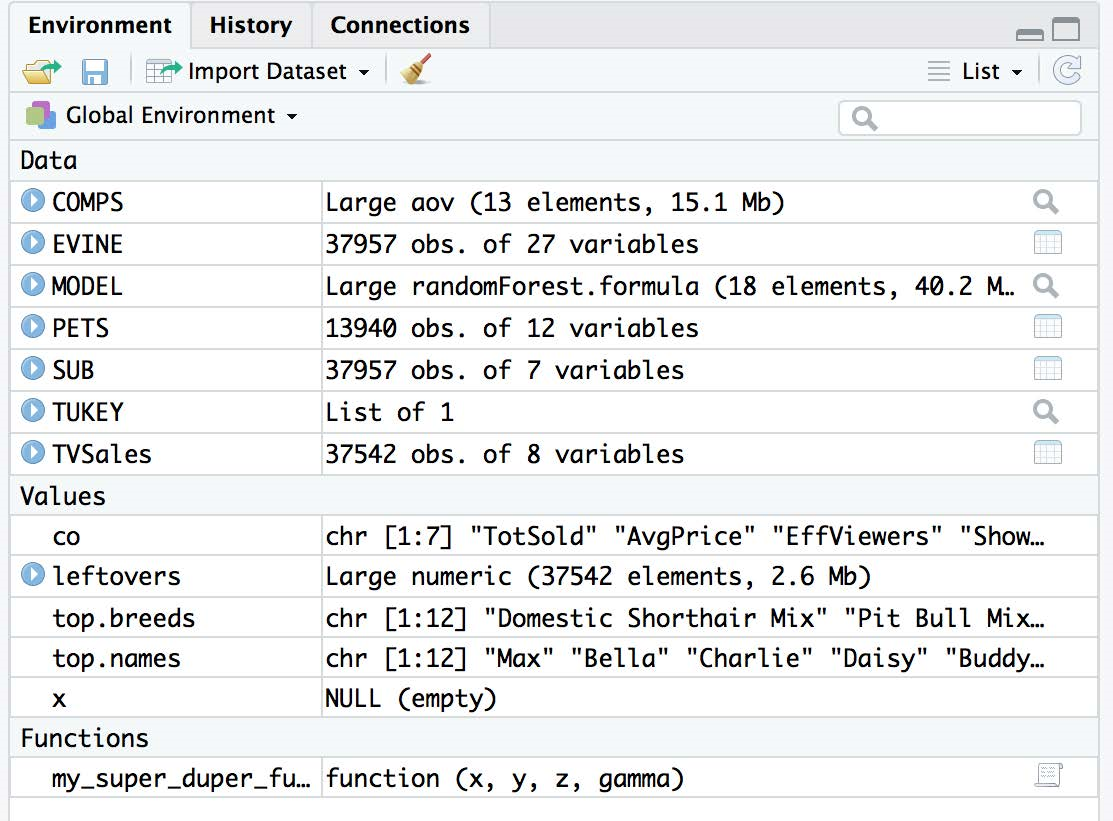
The upper-right window in RStudio gives a list of objects that are currently in the global environment (neatly split up by type: Data, Values, Functions, etc.).

As you will see shortly, functions run in their own, personal environment that is separate from the global environment.

When you quit and RStudio asks you if you want to ``save workspace image”, it is asking you if you would like to save a file that contains all objects that are defined in the global environment!

You can save your global environment by selecting from the top menu Session, Save Workspace As (and giving the file a name, which will have the extension .RDdata), and you can load previously saved global environments into the current R session by selecting Session, Load Workspace or by running \(load("filename")\).

You’ll be using the \(load\) function on your first take-home exam, since I will have created a global environment of dataframes and functions unique to you that you will use.

Basic Structure#

Like a loop, a function is essentially a shortcut for performing a bunch of commands. The basic structure of a function looks like:

function.name <- function(list of arguments separated by commas) {
  a bunch of code that does things  (body of function)
  #return the function output, e.g., a variable, dataframe ...
  return(something)
}

Note: the \(return\) statement is actually optional. By default, R will “return” whatever would be ``printed to the screen” (if anything) when executing the last line of the function.

What happens when a function is run#

add.two.numbers <- function(num1,num2) {
  temp <- num1+num2
  return(temp)
}
add.two.numbers(3,7)
#Running add.two.numbers(3,7) is a shortcut for the following lines of code
#First, R defines quantities based on the values of the arguments used
num1 <- 3
num2 <- 7
#Then, R runs the code in the function
temp <- num1+num2
#The return(temp) prints the contents of temp to the screen; 
# this output can be leftarrowed into a variable!

10

Quick note on the return statement#

If R runs the \(return\) statement in a function, the function terminates, even if there is code after the return!

ex.fun <- function(x) {
  if( length(x) == 1 ) { return(x) }
  #if length(x) is 1, function will terminate and code below doesn't run
  temp <- c()
  for (i in 2:length(x)) { temp[i] <- x[i]-x[i-1] }
  return(temp)
}

This function returns the differences in sequential elements of the vector \(x\), unless \(x\) only has one element (in which case it returns \(x\)). If \(x\) only has one element, then the \(return\) statement terminates the function and the lines of code below don’t run.

Returning multiple objects#

Functions can only ``return” a single object. Normally, this is fine because we often only want back a single number, a vector, or a dataframe. If you need to return more than one object (e.g., the min and the max of a vector, or a vector and a dataframe), you have to return a list.

info <- function(x) {
  n <- length(x)
  mean.value <- sum(x)/n; median.value <- median(x); sorted.values <- sort(x)
  result <- list(Mean=mean.value,Median=median.value,Sorted=sorted.values)
  return(result)
}
s <- info(c(9,4,1.3,6,7))
s$Mean; s$Median; s$Sorted

5.46

6

1.3
4
6
7
9

Names of objects passed to functions are irrelevant#

Even though a function takes an argument, e.g., \(x\), you do NOT need to make sure that you pass to the function an object with the same name. The function will treat what you passed as an argument correctly!

square.it <- function(x) { return(x^2) }
square.it(3)
#passing the argument as a value called 'a' won't mess up the function
a <- 3; square.it(a)

9

When the function is run, the mini-universe it creates will define an object called \(x\) (since the function is define with \(x\) as its first argument) and left-arrow it to the value passed to the function (in this case, whatever \(a\) happens to equal).

Setting default arguments#

It may be the case that one of the arguments you pass to a function is most likely always going to be some particular number. We can declare the function so that this argument takes on a default value unless it is specified otherwise. Simply use an equal sign to tell the function the default value!

#normally, distance = sqrt( (x[1]-y[1])^2 + (x[2]-y[2])^2 )
distance <- function(x,y,r=2) {#Euclidean distance between points when r=2
  temp <- (x-y)^r
  result <- sum(temp)^(1/r)
  return(result)
}
a <- c(1,2); b <- c(4,6)
distance(a,b)  #the argument r will default to equalling 2
distance(a,b,r=4) #the argument r is forced to equal 4

5

4.28457229495382

Order of arguments#

When a function takes multiple arguments, the argument order matters.

a <- c(1,2); b <- c(4,6)
distance(a,b,4)  #the argument r is forced to equal 4

4.28457229495382

R will define \(x\) to be \(a\) (since it appears first in the list of arguments), \(y\) to be \(b\), and \(r\) to be 4 (since it appears last in the list of argument).

However, you may put arguments in any order if you state their names in the function definition and use the equal sign to set them.

#function will define x,y,r as specified by arguments
distance(r=4,x=c(1,2),y=c(4,6))

4.28457229495382

Variables created inside a function cease to exist upon termination#

Functions are like Vegas: what happens in the function stays in the function. If you want to use something created in a function, it has to be returned!

raise.power <- function(x, n){
  temp1 <- x^n
  temp2 <- 1
  return(temp1+temp2)
}

Even though \(raise.power\) defines \(temp1\) and \(temp2\), these definitions only take place in the mini-universe, so their definition (or lack thereof) in the global environment remain unchanged after the function is run.

temp1 <- 1; temp1  #it's 1
raise.power(4,2)
temp1 #Still 1 even though it was redefined inside a function
temp2 #This value ceased to exist when function completed
n #n was defined to be 2 by the function arguments,
# but only in the miniuniverse not in the global environment

Writing your own functions#

The first rule in writing advanced code (loops, functions, etc.) is:

Note

Never try to write your function all in one go! The worst thing you can do is to start writing \(myfun <- function(arg1,arg2)\) etc., without knowing exactly what code is going to be in the body of the function! Write the body of your function first for a specific test case or example. Then, figure out how to generalize it so that it will work inside a function.

It’s tempting to jump right in and write everything all at once. When you’re proficient at coding this can be acceptable, but if you’re learning how to code it is a recipe for disaster (it makes debugging and verifying that your function is working monumentally difficult).

Guidelines for a good function#

A ``good” function has the following properties

The function name is not on the “reserve” list (i.e., already another R function). In other words, do not call your function \(c, mean, max, data\), etc.
Names of the function and variables should be somewhat informative so you can “read” what the function does.
Comments should be placed before the function declaration (and potentially in the body) to remind yourself and other users what the function and code is trying to do (use the hash tag #)

Advanced Functions#

\(sapply\) for vectors#

The \(sapply\) function returns a vector, each element of which is the result of applying another function to the corresponding input.

sapply(1:10, function(x)x^2)
sapply(1:ncol(airquality), function(col)mean(airquality[,col]))
colMeans(airquality)
sapply(1:ncol(airquality), function(col)mean(airquality[,col], na.rm=TRUE))
colMeans(airquality, na.rm=TRUE)

1
4
9
16
25
36
49
64
81
100

<NA>
<NA>
9.95751633986928
77.8823529411765
6.99346405228758
15.8039215686275

Ozone: <NA>
Solar.R: <NA>
Wind: 9.95751633986928
Temp: 77.8823529411765
Month: 6.99346405228758
Day: 15.8039215686275

42.1293103448276
185.931506849315
9.95751633986928
77.8823529411765
6.99346405228758
15.8039215686275

Ozone: 42.1293103448276
Solar.R: 185.931506849315
Wind: 9.95751633986928
Temp: 77.8823529411765
Month: 6.99346405228758
Day: 15.8039215686275

\(apply\) for data frames#

Very often, you may want to calculate the same function on the values in each ROW of a dataframe (e.g., each row is a customer and each column is the amount of money they have spent in different categories of items; you might want the sum of values to get the total they have spent).

Other times, you want want to calculate the same function on the values in each COLUMN of a dataframe (e.g., you want to calculate the fraction of missing values that are missing for each variable).

As long as all columns are numerical, the \(apply\) function allows you to do this quickly and efficiently (instead of having you write a \(for\) loop to go through each column or each row one by one).

\(apply\) syntax#

Syntax:

Note

\(apply(DATA,direction,FUN)\)

\(DATA\) is the name of the dataframe (each column must be numerical)
\(direction\) is either 1 (calculate the function for each row) or 2 (calculate the function for each column)
\(FUN\) is the name of the function (can be your own) that you want computed

Examples of functions applied to rows (direction is 1)#

GRADES <- data.frame(HW1=c(80,90,0),HW2=c(82,91,94),HW3=c(76,78,88))
apply(GRADES,1,sum) #total number of points achieved via homework
rowSums(GRADES) #same results
my.fun <- function(x) {
  x <- sort(x)[-1]  #take out the lowest score of x
  mean(x) #return the average of what's left
}
apply(GRADES,1,my.fun) #homework average after lowest score is dropped

238
259
182

238
259
182

81
90.5
91

Examples of functions applied to columns (direction is 2)#

#calculate the average value of each column
apply(airquality,2,mean)
colMeans(airquality) #same results
#number of values in each column that are NA
my.fun <- function(x) { sum(is.na(x)) }
apply(airquality,2,my.fun)
colSums(is.na(airquality)) #same results

Ozone: <NA>
Solar.R: <NA>
Wind: 9.95751633986928
Temp: 77.8823529411765
Month: 6.99346405228758
Day: 15.8039215686275

Ozone: <NA>
Solar.R: <NA>
Wind: 9.95751633986928
Temp: 77.8823529411765
Month: 6.99346405228758
Day: 15.8039215686275

Ozone: 37
Solar.R: 7
Wind: 0
Temp: 0
Month: 0
Day: 0

Ozone: 37
Solar.R: 7
Wind: 0
Temp: 0
Month: 0
Day: 0

The \(aggregate\) function#

You can imagine that if you wanted to find the average customer lifetime value for each combination of gender, income, state of origin, marital status, etc., this would be a phenomenal amount of nested \(for\) loops.

The good news is that since looking at the average (or median, proportion, etc.) for combination of groups is such a common task in analytics that R has a built-in function called \(aggregate\) that will quickly tabulate your function of interest for combinations that you specify.

The general syntax is \(aggregate(formula,DATA,FUN)\). The formula and FUN is used to specify what numerical value is to be calculated for groups, and the DATA argument just tells R where the columns are located.

\(aggregate\)#

The formula command is something akin to what you use when making a plot, fitting a regression, etc.

\(CLV \)\sim\( Gender\): will work with the distribution of CLV for each level of Gender
\(CLV \)\sim\( Gender + Married\): will work with the distribution of CLV for each combination of Gender and marital status (e.g., male/married, male/unmarried, female/married, female/unmarried)
\(CLV \)\sim\( .\): will work with the distribution of CLV for each combination of variables in the dataset (dangerous to use because this might be a LOT of combinations)
\(FirstP+LastP \)\sim\( Gender\): will work with the distribution of the sum of FirstP and LastP for each level of Gender
\(. \)\sim\( Gender\): will give the requested function on every quantitative variable in the data for each level of Gender

\(aggregate\) FUN#

The \(FUN=\) argument (yes, you have to capitalize it) tells it what function to calculate regarding the quantitative variable when considering each level of the categorical variable in the argument. You can even write your own functions!

\(FUN=mean\): will calculate the average value for each group
\(FUN=median\): will calculate the median value for each group
\(FUN=my.fun\): will calculate result of running \(my.fun\) (your own function you wrote) on the quantitative variable for each group.

\(aggregate\) examples#

library(regclass); data(CUSTLOYALTY)

#avg lifetime value for men/women
aggregate(CustomerLV~Gender,data=CUSTLOYALTY,FUN=mean)  
#avg lifetime value for each combo of gender/marital statusmen/women
aggregate(CustomerLV~Gender+Married,data=CUSTLOYALTY,FUN=mean)  
#summary of loyalty card for each gender
aggregate(LoyaltyCard~Gender,data=CUSTLOYALTY,FUN=summary)

A data.frame: 2 × 2
Gender	CustomerLV
<fct>	<dbl>
Female	1061.611
Male	1194.516

A data.frame: 4 × 3
Gender	Married	CustomerLV
<fct>	<fct>	<dbl>
Female	Married	1077.048
Male	Married	1222.587
Female	Single	1056.330
Male	Single	1185.005

A data.frame: 2 × 2
Gender	LoyaltyCard
<fct>	<int[,2]>
Female	79, 176
Male	74, 171

R: Functions

Contents

R: Functions#

Arguments#

Return#

Body#

Environment#

Basic Structure#

What happens when a function is run#

Quick note on the return statement#

Returning multiple objects#

Names of objects passed to functions are irrelevant#

Setting default arguments#

Order of arguments#

Variables created inside a function cease to exist upon termination#

Writing your own functions#

Guidelines for a good function#

Advanced Functions#

\(sapply\) for vectors#

\(apply\) for data frames#

\(apply\) syntax#

Examples of functions applied to rows (direction is 1)#

Examples of functions applied to columns (direction is 2)#

The \(aggregate\) function#

\(aggregate\)#

\(aggregate\) FUN#

\(aggregate\) examples#