Association Rules (Unsupervised Learning)#
Outline#
Four pillars of data mining#
Association rules (market basket analysis) - find commonly co-occurring traits. What grocery store items are often purchased together? What sets of movies are commonly enjoyed by the same individual? What web pages are useful given a search string? Descriptive analytics.
Clustering/Segmentation - find groups of individuals that are “similar” in some regard and ``cluster” though, though we don’t know ahead of time whether clusters exist or what they should even look like. For example, what market segments exist? The price-sensitive consumer, the die-hard fan, the early adopter, etc. Descriptive analytics.
Classification - given a set of training data and the ``answers” (actual classes of each individual), develop some model that is effective at predicting the class labels of as yet unseen individuals. Predictive analytics.
Numerical Prediction (Regression) - given a set of training data and the ``answers” (actual \(y\)-values of each individual), develop some model that is effective at predicting the \(y\) value of as yet unseen individuals. Predictive analytics.
Supervised vs. unsupervised learning#
Clustering and market basket analysis is more on the side of unsupervised learning since deals with finding patterns (e.g., clusters, rules, associations) that we may not even know exist. This field studies “unlabeled data”. There are no “answers” built-in to the data and nothing we can check in the data to verify our “discoveries” are correct; in fact we are trying to discover what an ``answer” even means.
Classification and Regression are supervised learning techniques. We have a target and our model is trying to hit it.
Association rules and clustering are unsupervised learning techniques because we don’t know what rules or clusters exist ahead of time.
Text mining, pattern mining, sentiment analysis, sequence mining (topics we will not discuss) sometimes blend the two together.
The outputs of an unsupervised learning procedure can potentially be used in supervised learning. For example, after market segmentation, a model could use the segment identity to predict customer lifetime value.
Motivation and Examples#
Certain items that shoppers buy often appear in the same transaction (``cart”)
Grocery: shoppers buy milk and eggs, toothpaste and mouthwash, or beer and diapers together
Netflix: viewers watch the trio of movies Inception, Minority Report, and Avatar quite frequently
amazon.com: surfers often look at the pages for Vitamin C serum, Hyaluric Acid Serum, and Micro Need Roller in the same session
What do we do with this info?
If there is a pair of items A and B (e.g., canned soup and sriracha sauce) that are frequently bought together:
Both A and B can be placed on the same shelf, so that buyers of one item would be prompted to buy the other.
Promotional discounts could be applied to just one of the two items.
Advertisements for product B could be targeted at buyers who have purchased product A.
A and B could be combined into a new product, such as having canned soup with a flavor of sriracha.
Companies are interested in what items go together so they can find combinations of products for special promotions or sales, devise a more effective store layout, and study brand loyalty and co-branding.
Barbie and candy#
Imagine Wal-Mart knows that customers who buy Barbie dolls (it sells one every 20 seconds) have a 60% chance of buying one of three types of candy bars. What does Wal-Mart do with information like that?
Extreme example: increase the price of a Barbie doll and give that type of candy bar for free. Wal-mart can reinforce the buying habits of that particular type of buyer.
Highest margin candy to be placed near dolls.
Special promotions for Barbie dolls with candy at a slightly higher margin.
Take a poorly selling product X and introduce an offer liked ``buy Barbie and her favorite candy and get Product X at 50% off”. If the customer is likely to buy these two products anyway then why not try to increase sales of X?
Introduce a bundle that contains not only a Barbie and Candy of type A, but also a new candy of Type N. The bundle is going to sell because of Barbie/Candy A, so candy of type N gets a free ride to customers houses. Candy of type N can become popular!
VHS players and recorders#
Electronics store did some early examples of association rule mining
Customers who buy a VHS player/recorder tend to come back to the store about 3-4 months later to buy a video camera (camcorder)
Store sends discount coupons for camcorders to all of its customers who bought VHS player/recorders a few months earlier, in order to bring those customers back into the store to purchase a camcorder
Temporal component to association rules can be key!
Wal-mart and hurricanes#
http://www.nytimes.com/2004/11/14/business/yourmoney/what-walmart-knows-about-customers-habits.html
In 2004, a series of hurricanes crashed into Florida. Wal-mart performed association analysis on what people purchased before the first one to intelligently plan what was needed for the others. What did customers really want the most prior to a hurricane?
They found one particular item that increased in sales by a factor of 7 over normal shopping days.
It wasn’t bottled water, batteries, beer (though that remains a best seller), flashlights, generators, or any of the usual things that we might imagine.
This item was ``discovered” by seeing what was associated with sales of beer.
The answer will surprise you!
The item was strawberry pop tarts! This might make sense.
No refrigeration or cooking
Individually wrapped portions
Long shelf life
Snack food, breakfast food
Kids love them, and we love them!
Despite these ``obvious” reasons, it was still a huge surprise! Walmart stocked their stores with tons of strawberry pop tarts prior to the next hurricanes, and they sold them out. That is a win-win: Walmart wins by making the sell, and customers win by getting the product that they most want.
You can play with some of the data here: https://www.kaggle.com/c/walmart-recruiting-sales-in-stormy-weather
Problem Statement#
Given a large transactional database (or data that can be thought of as one), how do we:
Find pairs, triplets, quadruplets, etc., of product that are appearing together in carts more often than chance alone would dictate?
Find rules that carry practical significance in terms of decision making?
Find rules that are surprising and/or insightful?
If a store carries 10,000 unique products (small-ish grocery store), then there are 49,995,000 pairs of products to analyze, 166,616,670,000 triplets of products to analyze, 416,416,712,497,500 quadruplets of products to analyze, and in general \(choose(10000,k)\) k-tuples of products to analyze.
How do we talk about rules that are being discovered? What makes a rule interesting? Useful? Let’s restrict ourselves to certain times of rules.
Note
Rule: if items \(X_1\), \(X_2\), \(X_3\), etc. are in the cart, then item \(Y\) may also be in the cart. This is abbreviated {\(X_1\), \(X_2\), \(X_3\) \(\rightarrow\) \(Y\)}.
Fundamentally, this is a rule about item Y and how likely it is to be in a cart when we know other items are already there.
Lift - Compared to the overall probability that \(Y\) is in the cart, how many times more likely is it that \(Y\) is in the cart once we know that items \(X_1\), \(X_2\), etc., are in the cart?
Confidence - What is the chance that the rule is correct? What fraction of carts with items \(X_1\), \(X_2\), etc. also do indeed have item \(Y\)?
Support - How prevalent or widely applicable is this rule? To what fraction of carts does this rule apply?
Support and Confidence#
In association rule mining we usually focus on rules in terms of their support and confidence.
Imagine that out of 10000 carts, 800 contains both items A and B. Of those 800, 100 contain item C as well. Our rule might be “{A,B} \(\rightarrow\) C”, i.e., ``if a cart has both items A and B in cart, then it may also have item C”.
Support - the fraction of transactions to which the rule applies, i.e., the fraction of carts that have all items mentioned in the rule. In this example, the rule {A,B} \(\rightarrow\) C has support 100/10000 = 0.01 (the number of transactions that contain items A, B, C divided by the total number of transactions).
Confidence - the fraction of transactions for which the rule is correct. The rule {A,B} \(\rightarrow\) C has confidence of 100/800 = 0.125 since 12.5% of carts with items A and B also have item C.
Goal: find rules with large lifts that also have large support (applicable to many transactions) and a high level of confidence (the rule is correct quite often)!
Towards Defining Lift - Probability of buying two items#
Let event A be a shopper having item A in cart and let event B be a shopper having item B in cart. Let \(P(A)\) and \(P(B)\) be the probabilities of the two events.
In general, the probability of both events occurring (i.e., a shopper has both items A and B in cart) is given by:
where \(P(A|B)\) the “conditional probability” of finding item A in the cart ``conditioned on the fact that” the shopper has item B in the cart.
Note
\(P(A|B)\) is read ``the probability of A, given B”. It is the probability that a shopper has item A given that the shopper already has item B in the cart.
If a shopper picks items at random (i.e., with a chance equal to the overall fraction of shoppers who buy each product), then the events of having items A and B are independent, so \(P(A|B) = P(A)\) and the probability of having both becomes:
Intuitively this makes sense. If the shopper picks items at random, then knowing that the shopper has item B gives us no indication of whether the shopper will also have item A.
These three quantities can be estimated from transactional data.
\(P(A)\) = fraction of carts containing item A. Also called the support of A.
\(P(B)\) = fraction of carts containing item B. Also called the support of B.
\(P(A \textrm{ and } B)\) = fraction of carts containing both items A and B (the support of the itemset AB)
When we discuss shoppers picking items or buying items “at random”, we don’t mean the shopper walks down the aisle, flips a coin at each product, then picks it if it comes up ``heads”.
``At random” means
with respect to the overall frequencies that shoppers buy the item and
that the chance of selecting a particular item is independent of what items are already present (and missing) from the cart.
For example, if 5% of shoppers buy item A, 1% of shoppers buy item B, and 25% of shoppers buy item C, then if Joe is picking items ``at random” there is a 5% chance he will pick item A, 1% chance he will pick item B, and a 25% he will pick item C (all independently of one another).
Lift - Quantifying the association#
If we find that \(P(A \textrm{ and } B) \approx P(A)P(B)\), then for all intents and purposes we can treat shoppers as picking these items independently from each other (their occurrence together is about as often as we’d expect if shoppers were picking items at random).
If we find that \(P(A \textrm{ and } B) \gg P(A)P(B)\), then we have evidence that items A and B are being picked together with a frequency much greater than what would be expected by chance. These are items that appear related!
The lift of a pair is defined to be:
Interpretation
Items A and B are found in carts together \(Lift\) times more often than what would be expected ``by chance” (i.e., if shoppers were picking items at random).
If item B is in the cart, the probability that A is in the cart increases by a factor of \(Lift\) (relative to the probability that a cart would have item A with no knowledge of what other items are in the cart).
If item A is in the cart, the probability that B is in the cart increases by a factor of \(Lift\) (relative to the probability that a cart would have item B with no knowledge of what other items are in the cart).
Note: the numerical value of the lift does not depend on the ``ordering” of the items (i.e., what is called item A and what is called item B).
Writing the formula in a slightly different way we get:
\(P(A)\) is the ``prior probability” that a cart will have item A
\(P(A|B)\) is the ``posterior probability” that a cart will have item A, given that item B is in the cart
We see that the Lift gives the factor by which the probability of finding item A in the cart has increased once we know that item B is in the cart.
Example: out of 1000 carts, toothpaste was found in 50, floss was found in 20, and both were found in 15.
\(P(toothpaste \textrm{ and } floss) = 15/1000\) = support(toothpaste + floss)
\(P(toothpaste) = 50/1000\) = support(toothpaste) and prior probability of finding toothpaste
\(P(floss) = 20/1000 = 0.02\) = support(floss) and prior probability of finding floss
\(Lift = (15/1000) / ( 20/1000 \cdot 50/1000 ) = 15\)
Toothpaste and floss are found together 15 times more often than what would be expected by chance (if shoppers were picking items at random). If toothpaste is in the cart, the probability that floss will also be there increases by a factor of 15 (from 0.02 to \(15 \times 0.02 =0.3\)).
Lift Interpretation#
Consider the rule: if \(X_1\), \(X_2\), etc., then \(Y\), i.e. {\(X_1\), \(X_2\) \(\rightarrow\) \(Y\) }. \(Y\) has a support (item frequency) of 0.015 and the rule has a lift of 16 (note that \(16 \times 0.015 = 0.24\)).
Note
The probability of finding item \(Y\) in the cart goes from 1.5% to 24% once we know that items \(X_1\) and \(X_2\)., are also in the cart.
A lift of 1 means the probability of finding \(Y\) is the same regardless of whether \(X_1\), \(X_2\), etc., are in the cart.
A lift less than 1 means that fewer carts than average have item \(Y\) when \(X_1\), \(X_2\), etc., are in the cart (``if Pepsi then Coke” would likely have a lift less than 1).
A lift greater than 1 means that more carts than average have item \(Y\) when \(X_1\), \(X_2\), etc., are in the cart (``if dry pasta then tomato sauce” would likely have a lift greater than 1). Larger values are typically more interesting and indicate stronger associations.
Depending on how often a certain item is purchased, there is a cap on the maximum value for the lift.
Imagine \(P(A)=0.5\) (half of shoppers have item A in their carts)
The maximum value of the lift is then 2, since \(Lift = P(A|B)/P(A) = P(A|B)/0.5 = 2P(A|B)\), and \(P(A|B)\) (like all probabilities) is at most 1.
In general, the maximum value of the lift involving item \(A\) is \(1/P(A) = 1/support(A)\).
Keep this in mind moving forward. For most of the examples we will consider, all items have a fairly small support so that the maximum values of their lifts are very large. However, it would be extremely interesting to see \(P(A)=0.7\) and \(P(A|B)=1\) (which would have a lift of 1.4), so be careful considering lift alone.
Imagine the rule ``If detergent and apple juice, then bananas” had a lift of 1.1. Normally, a lift of 1.1 isn’t interesting since bananas are only 1.1 times more likely to be in a cart (once we know detergent and apple are in it) than had we no knowledge of the other items in the cart.
But what if 90% of carts have bananas to begin with? That means that if we know that a cart has detergent and apple juice, the probability of it also having bananas increases from 90% to \(1.1 \times 90\) = 99%. That might be really quite interesting.
The trio of numbers for the support, confidence, and lift should be interpreted together. Here’s a pretty comprehensive interpretation of the rule ``if A and B then C”, taking the support of the rule to be 0.05, the support (item frequency) of C to be 0.10, the confidence of the rule to be 0.70, and the lift of the rule to be 7.
Note
Overall, 10% of carts contain item C (support of C). The probability of finding item C in a cart increases from 10% (support of C/prior probability) by a factor of 7 (lift) to 70% (confidence; lift times prior) among carts that contain items A and B. Indeed, if a cart has items A and B, there’s a 70% chance (confidence) it also has item C. 5% of all carts have these 3 items (support of rule). Items A, B, and C are appearing in carts 7 times more frequently than expected had shoppers picked items at random.
Apriori Algorithm#
Our goal is to find rules of the form:
Note
If { \(A_1\) } and { \(A_2\) } and \(\ldots\) and { \(A_k\) } then { \(B\) }.
Shorthand: \(\{ A_1, A_2, \ldots, A_k \} \rightarrow B\)
In other words, if a cart contains items \(A_1\), \(A_2\), \(\ldots\), \(A_k\), then it may also have item \(B\) (with a certain level of confidence).
Antecedents - the items in the “if” statement, also known as the left-hand side of the rule.
Consequent - the item in the “then” statement, also known as the right-hand side of the rule.
the length of a rule is the total number of items in the “if” statement (the antecedents) plus the item in the ``then” statement (the consequent).
We will restrict ourselves to finding only rules with one item in the “then” part of the rule, i.e., with one consequent.
When a transactional database has \(n\) items, there are a total of ``\(n\) choose \(k\)” possible combinations of \(k\) items.
#number of combinations of 2, 3, and 8 items from 10000 unique items
choose(10000,2); choose(10000,3); choose(10000,8)
There’s too many possible rules to consider, even when we write loops to exhaustively consider them all!
The key to narrowing down our search is to realize that if an itemset has a support that is below the threshold of interest, then all rules involving that itemset will have a support below the threshold as well and we can immediately eliminate them from consideration.
For example, imagine we are only interested in considering rules with a support of at least 0.01. If the support of the itemset { A, B } is 0.008 (below the threshold), we can immediately eliminate rules { A } \(\rightarrow\) { B }, { B } \(\rightarrow\) { A }, { A,B } \(\rightarrow\) { C }, { A,B,D,E } \(\rightarrow\) { G }, etc.
Imagine a transactional dataset has 5 unique items. A ``tree” of all combinations of items that might serve as the support for rules is generated. Lines connect itemsets that differ by one item (the addition or deletion of an item).
If we find that the support of the itemset { A,B } is below our set threshold (e.g., less than 0.01), then all itemsets that include those items will also be below the threshold and we can eliminate (``prune”) them from consideration.
When we do find frequent itemsets with the same number of items (e.g., CD and CE), then we consider more complex combinations of those by merging" or joining” them together. CD + CE \(\rightarrow\) CDE.
What we just described is the apriori algorithm (the main alternative is ECLAT). Assuming the data is stored in ``transactional form” (each row is a cart and the entries in a row are the items that appear in the cart), this algorithm is quite efficient (not necessarily fast) at finding association rules of arbitrarily long lengths by extending itemsets one item at a time.
The arules package in R#
Data representation and Inspect#
To find association rules with the \(arules\) package, the data needs to be in ``transactions” format – each row contains the items in a cart. There’s a special command \(read.transactions\) command to read in such files.
library(arules)
library(arulesViz)
library(datasets)
G <- read.transactions("groceries.csv", format = "basket", sep = ",", cols = NULL)
inspect(head(G,4) )
Loading required package: Matrix
Attaching package: ‘arules’
The following objects are masked from ‘package:base’:

    abbreviate, write
    items
[1] {citrus fruit,
     margarine,
     ready soups,
     semi-finished bread}
[2] {coffee,
     tropical fruit,
     yogurt}
[3] {whole milk}
[4] {cream cheese,
     meat spreads,
     pip fruit,
     yogurt}
A transactions object is a special way to store data. It is ``like” a data frame in that we can refer to rows with square brackets. However, in order to actually see any items or results we have to use the \(inspect\) command.
inspect(G[13:15])  #Carts 13-15
inspect(tail(G,2) ) #Last 2 carts
    items
[1] {beef}
[2] {frankfurter, rolls/buns, soda}
[3] {chicken, tropical fruit}
    items
[1] {bottled beer,
     bottled water,
     semi-finished bread,
     soda}
[2] {chicken,
     other vegetables,
     shopping bags,
     tropical fruit,
     vinegar}
You can make subsets of transactions that contain certain items.
#soda OR grape  (one or the other or both); use %in% shortcut
SUB <- subset( G,items %in% c("grapes","soda") )
inspect(SUB[c(12,10,5)])
#soda AND grade; use %ain$ shortcut (ONLY works for transactions)
SUB <- subset(G,items %ain% c("grapes","soda"))
inspect(SUB[c(26,18)])
    items
[1] {pastry, rolls/buns, soda}
[2] {grapes, ham, other vegetables, whole milk}
[3] {beef, detergent, grapes}
    items
[1] {berries, grapes, soda}
[2] {canned beer, grapes, other vegetables, soda}
Basic summary statistics#
Can get a visual of the most purchased items.
itemFrequencyPlot(G,topN=20,type="absolute",horiz=TRUE)
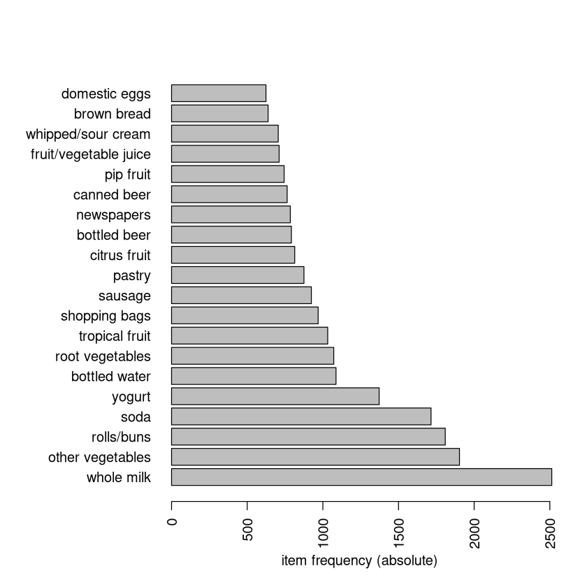
The \(itemFrequency\) command shows how often each item appears. These numbers are the supports of each item (prior probability of an item in the cart).
head(itemFrequency(G))  #First 6 supports alphabetically
itemFrequency(G)[121]; itemFrequency(G)["soups"]
- abrasive cleaner
- 0.00355871886120996
- artif. sweetener
- 0.0032536858159634
- baby cosmetics
- 0.000610066090493137
- baby food
- 0.000101677681748856
- bags
- 0.000406710726995424
- baking powder
- 0.017691916624301
length(G) #number of carts
length(G)*c(itemFrequency(G)[121],itemFrequency(G)["soups"])
- rice
- 75
- soups
- 67
In this example, rice appears in 0.76% of all carts (75 total) and soups appear in 0.68% of all carts (67 total).
Finding rules#
The example below shows how use \(apriori\) to record certain types of rules
minimum length of 2 (one item in the
if" part and one item in thethen” part)maximum length of 4 (three items in the
if" part and one item in thethen” part)support of at least 0.001 (at least 0.1% of carts must contain all items involved in the rule)
confidence of at least 80% (of the carts that contain the items in the “if” part of the rule, at least 80% also have the item in the ``then” part, i.e., the rule is correct for at least 80% of carts).
#Will always give a warning when you specify maxlen.
#This is simply letting us know it ran fine.
rules <- apriori(G, parameter = list(supp = 0.001, conf = 0.8, minlen=2,
                                     maxlen=4),control=list(verbose=FALSE))
To determine a ``reasonable” value for the support, think of how many carts are in the database. If you want the itemset to be in 1% of carts, then the support is 0.01. If you want the itemset to be in at least 100 carts and you have 42000, then the support is 100/42000 = 0.00238.
Confidence represents how often the rule is correct, so choose an appropriately high value (80% is usually the default)
Rules with a large maximum length are complex, hard to interpret, and may not have immediate or obvious practical use. Don’t make them too long. Also, compared to ``shorter rules”, rules with larger length may have higher confidence, but they will have smaller supports.
Once the rules object has been saved, you can use \(inspect\) (along with \(subset\) and some other commands) to print the rules out to the screen. By default, the rules appear in no particular order.
Note: I am going to set an option that makes R report only 3 digits instead of the default of 7. If you run this command, be sure at some point to chance this back to \(options(digits=7)\).
#changes the number of digits printed to the screen to 3.
#MUST CHANGE THIS BACK LATER
options(digits=3)  ; inspect(rules[1:5])
    lhs                         rhs            support confidence coverage
[1] {liquor, red/blush wine} => {bottled beer} 0.00193 0.905      0.00214
[2] {cereals, curd}          => {whole milk}   0.00102 0.909      0.00112
[3] {cereals, yogurt}        => {whole milk}   0.00173 0.810      0.00214
[4] {butter, jam}            => {whole milk}   0.00102 0.833      0.00122
[5] {bottled beer, soups}    => {whole milk}   0.00112 0.917      0.00122
    lift  count
[1] 11.24 19
[2]  3.56 10
[3]  3.17 17
[4]  3.26 10
[5]  3.59 11
The support, confidence, and lift of a rule are quality measures of the rule, and you can sort by any of them.
inspect(sort(rules, by="lift", decreasing=TRUE)[1:4] )
# inspect(sort(rules, by="confidence", decreasing=TRUE)[1:4] )
# inspect(sort(rules, by="support", decreasing=TRUE)[1:4] )
    lhs                         rhs              support confidence coverage  lift count
[1] {liquor,
     red/blush wine}         => {bottled beer}   0.00193      0.905  0.00214 11.24    19
[2] {citrus fruit,
     fruit/vegetable juice,
     grapes}                 => {tropical fruit} 0.00112      0.846  0.00132  8.06    11
[3] {butter,
     cream cheese,
     root vegetables}        => {yogurt}         0.00102      0.909  0.00112  6.52    10
[4] {pip fruit,
     sausage,
     sliced cheese}          => {yogurt}         0.00122      0.857  0.00142  6.14    12
Subsets of rules#
You can take a subset of rules that involve certain items. The \(\%in\%\) must be used instead of equality signs. Also, the \(\%ain\%\) is short for “all in” and it is useful for ensuring the carts have ALL the items listed.
CURD <- subset(rules, subset=lhs %in% "curd")#"if" statement must involve curd
inspect(sort(CURD, by="lift",dec=TRUE)[1:3] )
#"then" statement must involve whole milk or yogurt
DAIRY <- subset(rules, subset=rhs %in% c("whole milk","yogurt"))
inspect(DAIRY[c(156,153)])
    lhs                  rhs                support confidence coverage lift count
[1] {cream cheese,
     curd,
     root vegetables} => {other vegetables} 0.00173      0.850  0.00203 4.39    17
[2] {butter,
     curd,
     domestic eggs}   => {other vegetables} 0.00102      0.833  0.00122 4.31    10
[3] {curd,
     turkey}          => {other vegetables} 0.00122      0.800  0.00153 4.13    12
    lhs                 rhs          support confidence coverage lift count
[1] {butter,
     margarine,
     tropical fruit} => {yogurt}     0.00112      0.846  0.00132 6.07    11
[2] {bottled beer,
     domestic eggs,
     margarine}      => {whole milk} 0.00102      0.909  0.00112 3.56    10
#"if" statement must have meat AND root vegetables
STEW <- subset(rules, subset=lhs %ain% c("meat","root vegetables"))
inspect(STEW)  #only 1 rule
#LHS must have liquor and red/blush wine while the RHS must have bottled beer
ALCOHOL <- subset(rules,lhs %ain% c("liquor", "red/blush wine") &
                    rhs %in% "bottled beer")
inspect(ALCOHOL)
    lhs                                rhs                support confidence
[1] {meat, root vegetables, yogurt} => {other vegetables} 0.00122 0.857
    coverage lift count
[1] 0.00142  4.43 12
    lhs                         rhs            support confidence coverage lift
[1] {liquor, red/blush wine} => {bottled beer} 0.00193 0.905      0.00214  11.2
    count
[1] 19
You can also take a subset of rules that involve certain confidences, supports, or lifts.
important <- rules[quality(rules)$confidence > .99 & quality(rules)$lift > 3.5]
length(important)
inspect(important[1:3])
    lhs                                rhs          support confidence coverage
[1] {rice, sugar}                   => {whole milk} 0.00122 1          0.00122
[2] {canned fish, hygiene articles} => {whole milk} 0.00112 1          0.00112
[3] {butter, rice, root vegetables} => {whole milk} 0.00102 1          0.00102
    lift count
[1] 3.91 12
[2] 3.91 11
[3] 3.91 10
#we shortened the number of digits earlier, restore it back to default value
options(digits=7)
Visualizations#
The ``two-key” plot shows the prevalence of a rule (its support) versus its probability of being correct (confidence) broken down by lift (you can choose other ways to shade, such as the length of the itemset, confidence, etc). As is almost always the case, rules that are potentially more applicable because of their larger support tend to have lower confidence.
plot(rules, shading="lift", control=list(main ="Two-key plot"));
To reduce overplotting, jitter is added! Use jitter = 0 to prevent jitter.

The “grouped matrix” plot can show relationships between rules. Below, the rule implying the purchase of bottled beer has a large support, large lift, and only involve liquor (plus one other item) in the “if” statement. Only one rule has tropical fruit in the “then” part, while many rules imply the purchase of other vegetables.
plot(rules, method="grouped")

Perhaps the most fun plot is the graph of the rules where you can move around the nodes to make the presentation more clear. Note: interaction is not available on every computer.
simplerules <- apriori(G, parameter=list(supp=0.001,conf=0.7,maxlen=3),
                       control=list(verbose=FALSE))
#selecting some for illustration
simplerules <- sort(simplerules,by="lift")[ c(1:13,22:23,98) ]
plot(simplerules, method="graph", vertex.size=5, vertex.label.cex=0.6,
     control=list(type="items"), interactive=TRUE)
inspect(  simplerules  )
     lhs                               rhs                support confidence lift
[1]  {liquor,red/blush wine}        => {bottled beer}     0.00193 0.905      11.24
[2]  {grapes,onions}                => {other vegetables} 0.00112 0.917       4.74
[3]  {hard cheese,oil}              => {other vegetables} 0.00112 0.917       4.74
[4]  {butter milk,pork}             => {other vegetables} 0.00183 0.857       4.43
[5]  {coffee,misc. beverages}       => {soda}             0.00102 0.769       4.41
...
[13] {onions,sliced cheese}         => {other vegetables} 0.00153 0.789       4.08
[14] {rice,sugar}                   => {whole milk}       0.00122 1.000       3.91
[15] {canned fish,hygiene articles} => {whole milk}       0.00112 1.000       3.91
[16] {honey}                        => {whole milk}       0.00112 0.733       2.87
How to read the graph. Items that have an arrow coming out of it are involved in the left-hand side (“if” statement) of a rule. Items that have an arrowing pointing towards it are involved in the right-hand side (``then” statement) of a rule.
An arrow emerging from an item will point towards a circle. If any other item has an arrow pointing towards that same circle, then all those items are involved in the “if” part of the rule. The item pointed to by the arrow emerging from the circle is the item in the ``then” part of the rule.
Blue star: an arrow comes out of honey and points to a circle. Since it is the only arrow pointing to the circle, and the arrow coming out of the circle points to whole milk, the rule is { honey } \(\rightarrow\) { whole milk }.
Red start: an arrow comes out of margarine and points to a circle. The arrow from meat points to the same circle, and the arrow out of the circle points to other vegetables. The rule is { margarine, meat } \(\rightarrow\) { whole milk }.
Examples#
The transactional data is named \(G\) which has 9835 carts. Let’s have rules apply to at least 25 carts (support at least 25/9835) and have a level of confidence of at least 80% and a length of at most 5. Actually only 3 rules are found!
RULES <- apriori(G, parameter = list(supp = 25/9835, conf = 0.80, minlen=2,
                                     maxlen=5),control=list(verbose=FALSE))
length(RULES)
inspect(RULES)
    lhs                   rhs                    support confidence    coverage     lift count
[1] {curd,
     hamburger meat}   => {whole milk}       0.002541942  0.8064516 0.003152008 3.156169    25
[2] {curd,
     domestic eggs,
     other vegetables} => {whole milk}       0.002846975  0.8235294 0.003457041 3.223005    28
[3] {citrus fruit,
     root vegetables,
     tropical fruit,
     whole milk}       => {other vegetables} 0.003152008  0.8857143 0.003558719 4.577509    31
We need to start out by finding what fraction of carts have the RHS items.
itemFrequency(G)[c("whole milk","other vegetables")]
- whole milk
- 0.255516014234875
- other vegetables
- 0.193492628368073
These are not rare items. Whole milk is found in about 25% of carts and other vegetables in about 19%. However, this probability increases when we know some other items are in the cart! For example:
inspect(RULES[1])
    lhs                       rhs          support     confidence coverage
[1] {curd, hamburger meat} => {whole milk} 0.002541942 0.8064516  0.003152008
    lift     count
[1] 3.156169 25
Overall, the probability that a cart contains whole milk is 25.56%. However, among carts that have curd and hamburger meat, the probability that the cart has whole milk increases by a factor of 3.16 (the lift) to 80.6% (the confidence). A total of 25 carts (0.285% of the 9835 carts) have these three items together.
Additional Considerations#
Spurious Associations#
A spurious association is a “false positive” of sorts: an association rule that ``looks” important but that has been generated by chance (the items involved have no true association between them). This can be a problem for large datasets.
Analysis of large inventories involve more itemset configurations. Weak, but interesting, associations may require that the support threshold be quite low. However, lowering the support threshold also increases the number of spurious associations detected.
Same as what we did when constructing models for predictive analytics, we want the rules to be generalizable. Depending on the data and the problem, it may be useful to discover rules on a training data and assess their confidence on a holdout sample.
Drawbacks of the apriori algorithm#
The apriori algorithm has been immensely useful in business and many other disciplines. However, the algorithm does have drawbacks:
The number of rules obtained can be immense.
Many rules are not “interesting” or of direct practical use. “Interesting” is in the eye of the beholder, and it’s difficult to tell any algorithm what you find important. Having a stuff for lift, confidence, and support is about the best you can do (along with narrowing down the left/right hand side of the rules).
Although the algorithm does find rules in a clever way, it is quite slow for very large datasets.
Thinking about Interestingness#
In general what does it mean for a rule to be ``interesting”?
Unexpectedness - Rules are interesting if they are unknown to the user or contradict the user’s existing knowledge.
Actionability - Rules are interesting if users can do something with them to their advantage.
Actionable rules can be either expected or unexpected, but the latter are the ``most interesting” because they lead to more valuable decisions (decisions that were probably not going to be made without the analysis).
Most of the approaches for finding interesting rules in a subjective way require user input and participation so that the appropriate knowledge or goal into the analysis.
What do we do with interesting rules?#
What do we do with ``interesting” rules? It takes creativity, but let’s think through a few examples.
Imagine \(A, B \rightarrow C\), and \(C\) is a new item. Clearly, shoppers that like A and B also like item C, so find the shoppers who are buying A and B but who haven’t bought C yet (maybe they don’t know about it) and send them coupons for C. This is your chance to ``turn them on” to this product.
Imagine \(A, B \rightarrow C\), and that this rule has a fairly large support. These items are very frequently purchased together. Don’t discount them all at once because that’s throwing away money!
Imagine \(A, B \rightarrow C\), and that we want to get rid of item \(C\) with little regard to lost profits. Design a promotion that encourages buying \(C\)! Perhaps 50% off \(C\) if you buy items \(A\) and \(B\).
Reminder to be cautious#
When doing association rule mining, be careful.
A large lift doesn’t automatically mean the rule is legitimate. The value is tied into sample sizes, so check the support and confidence as well. Also check the statistical significance with the \(p\)-value adjusted based on the number of rules.
For popular items, there is a cap on the maximum value of the lift. A lift of 1.25 normally doesn’t get too much attention, but if the support of the RHS of the rule is 0.8, that means the probability of buy that item, given the items in the LHS, is now 100%.
Translate between the support of an itemset and the number of carts in your data. A lift of 34.2 and a confidence of 100% sounds impressive, but if this rule applied to only 3 carts out of 100,000 in the data it’s probably not useful.
Many rules are redundant. A simpler rule (fewer items involved) with at least as high a level of confidence takes precedence of a more complex rule.
Association rules are not physical laws. A rule that has 100% confidence doesn’t mean that if we coerce someone to buy the items in the “if” statement then they will also buy the item in the ``then” statement.