Neural Networks and Deep Learning

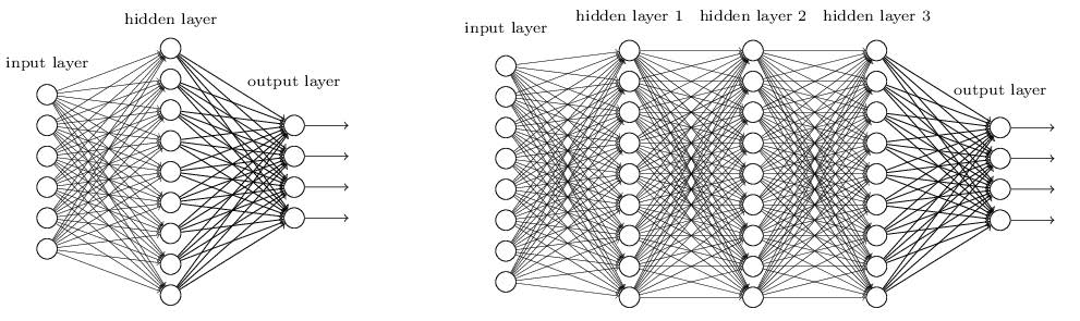
Neural Networks and Deep Learning#

Neural network models emerged from early attempts to model how neurons in the brain might work. While they have had only limited success in actually modeling anything biological and their popularity has ebbed and flowed (mostly due to computational limitations over time), they have become quite useful in machine learning.

In fact, you may have heard of the phrase ``deep learning”, which is used to solve problems in speed recognition, imagine recognition, 3-D object recognition. Deep learning is just a very large, very complex neural network.

So how does it work?

In 1958, Frank Rosenblatt developed the perceptron (in a sense is the most primitive neural network) to make classifications.

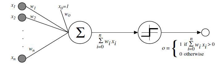
The perceptron takes input \(x_1\), \(x_2\), etc. (the values of predictor variables) and calculates the weighted sum \(w_0 + w_1 x_1 + w_2 x_2 + \ldots\), where weights can be positive or negative. However, it outputs either a 0 or a 1, depending on whether the value of the weighted sum is positive or negative.

If you think the process of making a prediction with the perceptron sounds like linear regression, you’re right.

\[ Regression = \beta_0 + \beta_1 x_1 + \beta_2 x_2 + \ldots \]

\[\begin{split} Perceptron = \begin{cases} 0 & if w_0 + w_1 x_1 + w_2 x_2 + \ldots \le 0 \\ 1 & if w_0 + w_1 x_1 + w_2 x_2 + \ldots > 0 \end{cases} \end{split}\]

In fact, the perceptron looks a lot like a linear regression model trying to predict the probability of a level and then classifying accordingly. Linear regression is usually a pretty bad model for this application (which is why we use logistic regression instead).

Activation Function#

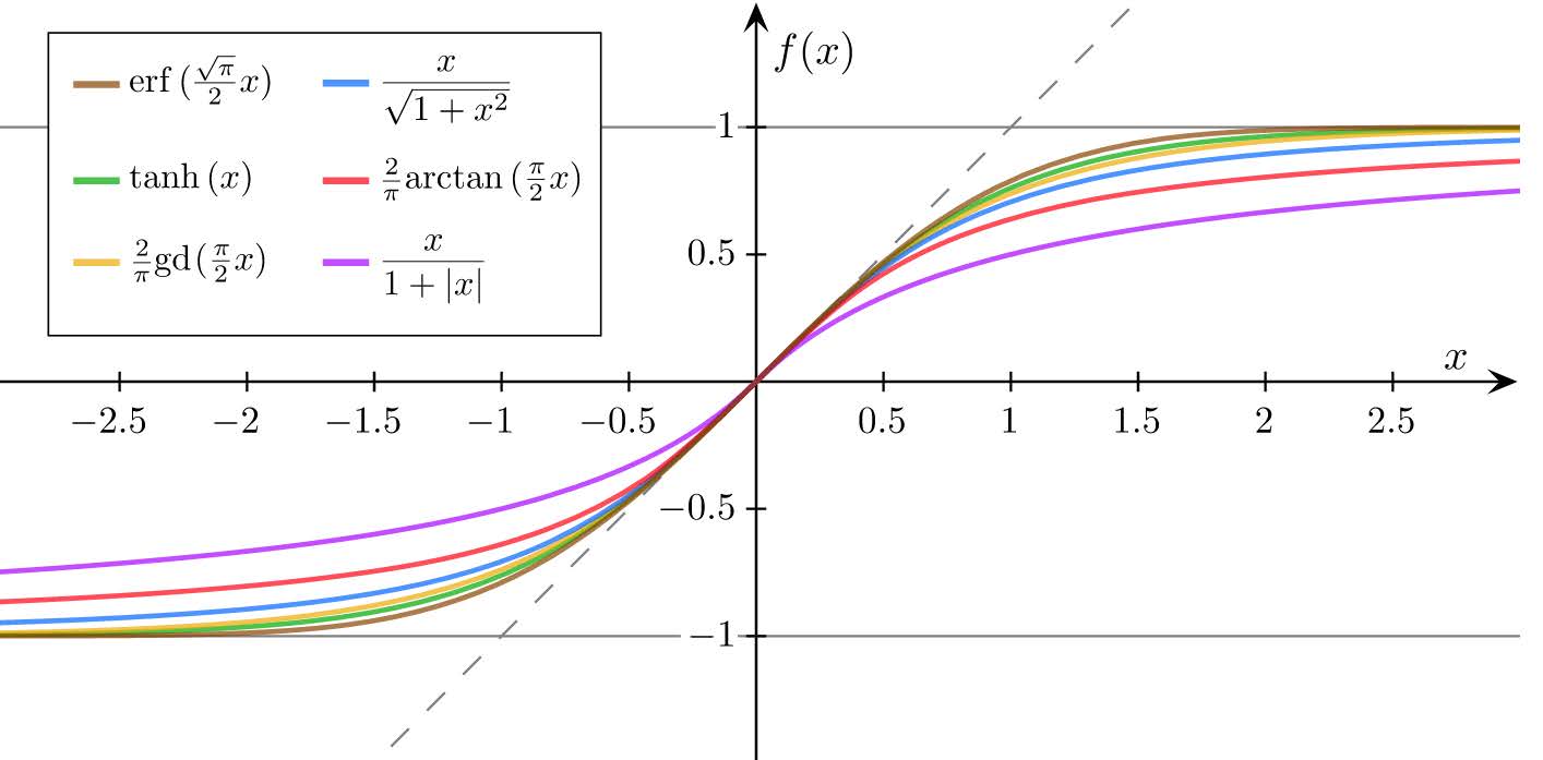
People realized that instead of transforming the weighted sum of predictors to an output using a ``step function” (0 if less than some threshold, 1 if greater), a better idea would be to feed the weighted sum into a more general activation function. One popular choice is the logistic function.

\[z = w_0 + w_1 x_1 + w_2 x_2 + \ldots\]

\[y = \frac{e^z}{1+ e^z} = \frac{1}{1 + e^{-z}}\]

When the perceptron uses the logistic activation function, the end result is logistic regression, which we can use the model the probability an individual possesses one of two classes.

By taking the weighted sum of predictor variables and passing it through the logistic activation function, the output becomes a number between 0 and 1 and could be interpreted as a probability. The upshot has been the logistic regression has been re-invented.

There are many choices of activation functions, though by far the most common is the logistic (aka sigmoid) due to some ``nice” theoretical properties.

../_images/2275e899dedbedaaa35bee75890bb4df9392e7406e627690b70dbe7ca9a3c0d7.png

There’s not a huge variety in what activation functions look like.

Hidden Layer#

The model is greatly improved by adding what’s known as a hidden layer.

Each neuron in the hidden layer received a weighted sum of predictor variables (each one receives a different sum), then outputs an ``activated sum” (e.g., passing it through the logistic function).
Whereas the perceptron uses the output from the activation function as the predicted value of \(y\), these outputs in the intermediate layer (the hidden layer) are essentially used as new predictor variables.
A weighted sum of these new predictor variables is created, run through one more activation function and transformed, and the output is finally the predicted value of \(y\).
The hidden layer is where this ``feature engineering” (variable creation) takes place. It constructs better predictors of \(y\) from the measured variables.

Imagine forecasting what will happen to a medical patient. A neural network would create weighted sums of predictor variables like age, sex, BMI, properties of a tumor and run them through a hidden layer to transform them into new predictors, which are then combined in a weighted sum to make the prognosis. Note: the Bias in this picture is analogous to the ``intercept” term in a regression (weighted sum of predictors, plus a numeric constant).

Multiple Hidden Layers (Deep Learning)#

Multiple hidden layers can be added to a neural network. They all work the same: transforming a weighted sum of inputs via an activation function and outputting the result. In effect, each hidden layer helps to improve on the transformations made of the layer before it, so it’s ``like” a boosted tree in that sense.

Deep learning means having a neural network with many hidden layers. As you can imagine, figuring out the correct weights in the weighted sums can be a complex, computationally intensive task.

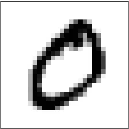
Example: MNIST Digits#

How do you personally figure out what digit is what? What features do you look for?

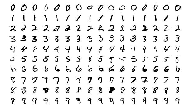
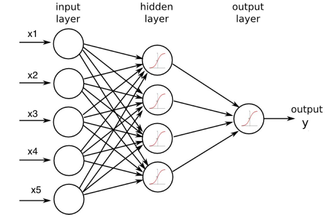
The hidden layer in the neural network might ``construct” features like:

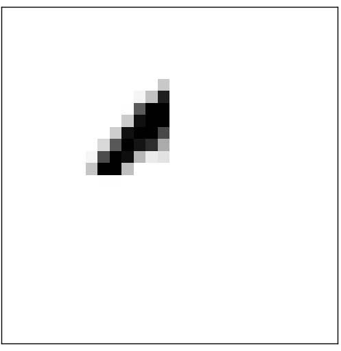
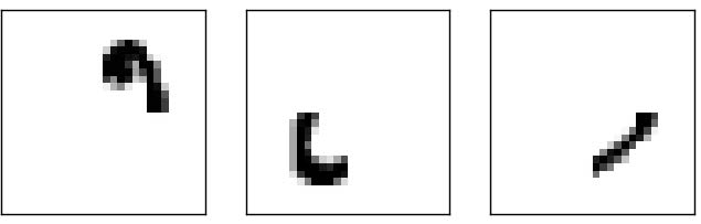
A ``weighted sum” of those four features could easily produce a 0! Other sets of features would be able to produce other digits.

Tuning Parameters#

When building a neural network for predictive modeling, you need to design it:

Number of hidden layers: More layers = lower bias (fitting the training data well) but larger variance and larger risk of overfitting unless you have a really big dataset.
Number of neurons in each hidden layer: essentially, the number of new variables to create from the original predictors. More neurons = lower bias but larger variance and larger risk of overfitting.
“Weight decay” (regularization): penalty given to large weights in the weighted sum to prevent overfitting and to improve generalization. This will prevent any particular predictor/feature from contributing “too much” and makes the model somewhat less sensitive to the set of individuals in the training data. Small weights make the modeled relationships “more linear” and prevents crazy curviness that may be unique to the training set. Not all implementations of the algorithm have this parameter.

Example and Pros and Cons#

The \(neuralnet\) lets us explore some aspects of the neural network model (we will not be using it for \(train\)), but the data frame has to have categorical variables converted to indicator variables and each variable needs to be scaled.

data(TIPS, package='regclass')
#Replace categorical variables with indicator variables (using only some of the predictors here)
DATA <- model.matrix(~TipPercentage+Bill+Gender+Smoker+PartySize,data=TIPS)[,-1]
#Create variables to store the mean and standard deviation of the y variable; need those later
mean.y <- mean(TIPS$TipPercentage); sd.y <- sd(TIPS$TipPercentage) 
DATA <- scale(DATA)  #Scale the data
NNET <- neuralnet(TipPercentage~Bill+GenderMale+SmokerYes+PartySize,data=DATA,
                  hidden=3,linear.output = TRUE,stepmax=1e6)

The \(hidden\) argument tells it how many neurons in the hidden layer (can make this a vector to add more hidden nodes). \(stepmax\) dictates how many search steps the algorithm is allowed to take to find the optimal set of weights.

Visualizing the neural network with neuralnet#

Warning: you may not be able to knit the plot of a neural network because of some odd choices the authors of the package made with the plot syntax (in fact, there is some chance your computer may not even be able to make the plot at all).

plot(NNET,rep="best")

../_images/e7acec67751dbdba6328b018106eb9c6cec074df4d43330917027f913a3f88b6.png

Making predictions with neuralnet#

The writers of the \(neuralnet\) package also decided to make their neural network model incompatible with \(predict\). Instead, you must use \(compute\).

Note: when giving it a dataset on which to make predictions, the columns must match up exactly with the columns used to train the model (unlike every other model we’ve discussed). The example below uses everything but the TipPercentage column (since that is the \(y\) variable and not an \(x\) variable that appears in the predictor matrix).

predictions.nnet <- as.numeric( compute(NNET,DATA[,-1])$net.result )  #ie without column of y
predictions.nnet <- predictions.nnet*sd.y + mean.y  #unscale
#RMSE on training data; not the most interesting
sqrt( mean( (TIPS$TipPercentage - predictions.nnet)^2 ) )  

4.72070819670374

Examples with \(tidymodels\)#

Example: neural networks (classification)#

data(EX6.WINE, package='regclass')

# This is not usually right if want to investigate testing performances.
TRAIN <- EX6.WINE

REC <- recipe(Quality ~ ., TRAIN) %>%
    step_normalize(all_numeric_predictors()) %>%
    step_dummy(all_nominal_predictors()) %>%
    step_nzv(all_predictors()) %>%
    step_corr(all_predictors()) %>%
    step_lincomb(all_predictors())

WF <- workflow() %>%
    add_recipe(REC) %>%
    add_model(mlp( mode = 'classification', hidden_units = tune(), penalty = tune() ))

GRID <- expand.grid( hidden_units = 1:7, penalty = 10^seq(-2,2,length=20) )

RES <- WF %>%
    tune_grid(
        resamples = vfold_cv(TRAIN, v = 5),
        grid = GRID,
    )

METRICS <- collect_metrics(RES)

METRICS

A tibble: 420 × 8
hidden_units	penalty	.metric	.estimator	mean	n	std_err	.config
<int>	<dbl>	<chr>	<chr>	<dbl>	<int>	<dbl>	<chr>
1	0.01000000	accuracy	binary	0.8188889	5	0.004771888	Preprocessor1_Model001
1	0.01000000	brier_class	binary	0.1615436	5	0.002081009	Preprocessor1_Model001
1	0.01000000	roc_auc	binary	0.8960086	5	0.006585751	Preprocessor1_Model001
2	0.01000000	accuracy	binary	0.8437037	5	0.007041909	Preprocessor1_Model002
2	0.01000000	brier_class	binary	0.1509120	5	0.002011134	Preprocessor1_Model002
2	0.01000000	roc_auc	binary	0.9148295	5	0.005190027	Preprocessor1_Model002
3	0.01000000	accuracy	binary	0.8451852	5	0.013902463	Preprocessor1_Model003
3	0.01000000	brier_class	binary	0.1482455	5	0.003201304	Preprocessor1_Model003
3	0.01000000	roc_auc	binary	0.9179203	5	0.007189008	Preprocessor1_Model003
4	0.01000000	accuracy	binary	0.8388889	5	0.004721314	Preprocessor1_Model004
4	0.01000000	brier_class	binary	0.1491965	5	0.001408213	Preprocessor1_Model004
4	0.01000000	roc_auc	binary	0.9150855	5	0.005121324	Preprocessor1_Model004
5	0.01000000	accuracy	binary	0.8555556	5	0.007790994	Preprocessor1_Model005
5	0.01000000	brier_class	binary	0.1403109	5	0.001886026	Preprocessor1_Model005
5	0.01000000	roc_auc	binary	0.9287602	5	0.005023629	Preprocessor1_Model005
6	0.01000000	accuracy	binary	0.8503704	5	0.007300149	Preprocessor1_Model006
6	0.01000000	brier_class	binary	0.1433502	5	0.002394401	Preprocessor1_Model006
6	0.01000000	roc_auc	binary	0.9222099	5	0.006045245	Preprocessor1_Model006
7	0.01000000	accuracy	binary	0.8525926	5	0.009633190	Preprocessor1_Model007
7	0.01000000	brier_class	binary	0.1420321	5	0.003782513	Preprocessor1_Model007
7	0.01000000	roc_auc	binary	0.9206950	5	0.007970750	Preprocessor1_Model007
1	0.01623777	accuracy	binary	0.8188889	5	0.005629142	Preprocessor1_Model008
1	0.01623777	brier_class	binary	0.1616034	5	0.002086724	Preprocessor1_Model008
1	0.01623777	roc_auc	binary	0.8959839	5	0.006575368	Preprocessor1_Model008
2	0.01623777	accuracy	binary	0.8362963	5	0.007444352	Preprocessor1_Model009
2	0.01623777	brier_class	binary	0.1538296	5	0.001384560	Preprocessor1_Model009
2	0.01623777	roc_auc	binary	0.9052567	5	0.002742090	Preprocessor1_Model009
3	0.01623777	accuracy	binary	0.8362963	5	0.006186405	Preprocessor1_Model010
3	0.01623777	brier_class	binary	0.1496267	5	0.002705010	Preprocessor1_Model010
3	0.01623777	roc_auc	binary	0.9153666	5	0.007604319	Preprocessor1_Model010
⋮	⋮	⋮	⋮	⋮	⋮	⋮	⋮
5	61.58482	accuracy	binary	0.7577778	5	0.0115410640	Preprocessor1_Model131
5	61.58482	brier_class	binary	0.2138267	5	0.0011151672	Preprocessor1_Model131
5	61.58482	roc_auc	binary	0.8449092	5	0.0061148461	Preprocessor1_Model131
6	61.58482	accuracy	binary	0.7674074	5	0.0098444695	Preprocessor1_Model132
6	61.58482	brier_class	binary	0.2127550	5	0.0010660400	Preprocessor1_Model132
6	61.58482	roc_auc	binary	0.8453169	5	0.0060603434	Preprocessor1_Model132
7	61.58482	accuracy	binary	0.7718519	5	0.0086741025	Preprocessor1_Model133
7	61.58482	brier_class	binary	0.2120647	5	0.0010521195	Preprocessor1_Model133
7	61.58482	roc_auc	binary	0.8455773	5	0.0060577024	Preprocessor1_Model133
1	100.00000	accuracy	binary	0.6074074	5	0.0124363951	Preprocessor1_Model134
1	100.00000	brier_class	binary	0.2368593	5	0.0009043861	Preprocessor1_Model134
1	100.00000	roc_auc	binary	0.8310725	5	0.0056761244	Preprocessor1_Model134
2	100.00000	accuracy	binary	0.6074074	5	0.0124363951	Preprocessor1_Model135
2	100.00000	brier_class	binary	0.2357033	5	0.0009584880	Preprocessor1_Model135
2	100.00000	roc_auc	binary	0.8297361	5	0.0056658875	Preprocessor1_Model135
3	100.00000	accuracy	binary	0.6074074	5	0.0124363951	Preprocessor1_Model136
3	100.00000	brier_class	binary	0.2357781	5	0.0009893254	Preprocessor1_Model136
3	100.00000	roc_auc	binary	0.8286669	5	0.0056627580	Preprocessor1_Model136
4	100.00000	accuracy	binary	0.6074074	5	0.0124363951	Preprocessor1_Model137
4	100.00000	brier_class	binary	0.2357890	5	0.0012697318	Preprocessor1_Model137
4	100.00000	roc_auc	binary	0.8284353	5	0.0058590361	Preprocessor1_Model137
5	100.00000	accuracy	binary	0.6074074	5	0.0124363951	Preprocessor1_Model138
5	100.00000	brier_class	binary	0.2347382	5	0.0011317313	Preprocessor1_Model138
5	100.00000	roc_auc	binary	0.8288569	5	0.0056654048	Preprocessor1_Model138
6	100.00000	accuracy	binary	0.6074074	5	0.0124363951	Preprocessor1_Model139
6	100.00000	brier_class	binary	0.2345973	5	0.0011312843	Preprocessor1_Model139
6	100.00000	roc_auc	binary	0.8286722	5	0.0056750661	Preprocessor1_Model139
7	100.00000	accuracy	binary	0.6074074	5	0.0124363951	Preprocessor1_Model140
7	100.00000	brier_class	binary	0.2343394	5	0.0011876321	Preprocessor1_Model140
7	100.00000	roc_auc	binary	0.8287848	5	0.0056720982	Preprocessor1_Model140

for(metric in unique(METRICS$.metric)){
    metrics <- METRICS %>% filter(.metric==metric)
    plot <- ggplot(metrics, aes(x=penalty, y=mean, color=as.factor(hidden_units))) + geom_line() + scale_x_log10() + labs(title=metric)
    print(plot)
}

../_images/561974c0df24305c7eea3d566836468f0fc385944887a4e334eb332b5d99998c.png

../_images/5768fd170e50f66ae6a3c44157dc6638ecae2568e45b9ce39130f9a2119ebcc2.png

../_images/53a524dea0e6b7d9d7e922d4267e0e056119dd2c22b469379066c6347c845e63.png

BEST <- select_best(RES, metric = 'accuracy')
BEST

A tibble: 1 × 3
hidden_units	penalty	.config
<int>	<dbl>	<chr>
7	0.1128838	Preprocessor1_Model042

MODEL <- WF %>%
    finalize_workflow(BEST) %>%
    fit(TRAIN)
MODEL

══ Workflow [trained] ══════════════════════════════════════════════════════════════════════════════════════════════════════════════════════════════════════════════════════════════════════════════════════════════
Preprocessor: Recipe
Model: mlp()

── Preprocessor ────────────────────────────────────────────────────────────────────────────────────────────────────────────────────────────────────────────────────────────────────────────────────────────────────
5 Recipe Steps

• step_normalize()
• step_dummy()
• step_nzv()
• step_corr()
• step_lincomb()

── Model ───────────────────────────────────────────────────────────────────────────────────────────────────────────────────────────────────────────────────────────────────────────────────────────────────────────
a 11-7-1 network with 92 weights
inputs: fixed.acidity volatile.acidity citric.acid residual.sugar free.sulfur.dioxide total.sulfur.dioxide density pH sulphates alcohol chlorides_Lots 
output(s): ..y 
options were - entropy fitting  decay=0.1128838

Example: neural networks (regression)#

data(EX9.BIRTHWEIGHT, package='regclass')

# This is not usually right if want to investigate testing performances.
TRAIN <- EX9.BIRTHWEIGHT

REC <- recipe(Birthweight ~ ., TRAIN) %>%
    step_normalize(all_numeric_predictors()) %>%
    step_dummy(all_nominal_predictors()) %>%
    step_nzv(all_predictors()) %>%
    step_corr(all_predictors()) %>%
    step_lincomb(all_predictors())

WF <- workflow() %>%
    add_recipe(REC) %>%
    add_model(mlp( mode = 'regression', hidden_units = tune(), penalty = tune() ))

GRID <- expand.grid( hidden_units = c(2,3), penalty = 10^seq(-2,1,length=15) )

RES <- WF %>%
    tune_grid(
        resamples = vfold_cv(TRAIN, v = 5),
        grid = GRID,
    )

METRICS <- collect_metrics(RES)

METRICS

→ A | warning: A correlation computation is required, but `estimate` is constant and has 0 standard deviation, resulting in a divide by 0 error. `NA` will be returned.

There were issues with some computations   A: x1

There were issues with some computations   A: x1

A tibble: 60 × 8
hidden_units	penalty	.metric	.estimator	mean	n	std_err	.config
<dbl>	<dbl>	<chr>	<chr>	<dbl>	<int>	<dbl>	<chr>
2	0.01000000	rmse	standard	500.34200416	5	27.78098862	Preprocessor1_Model01
2	0.01000000	rsq	standard	0.11557329	5	0.05032802	Preprocessor1_Model01
3	0.01000000	rmse	standard	514.41492660	5	25.03946676	Preprocessor1_Model02
3	0.01000000	rsq	standard	0.07509909	5	0.02697816	Preprocessor1_Model02
2	0.01637894	rmse	standard	492.35315438	5	19.92295040	Preprocessor1_Model03
2	0.01637894	rsq	standard	0.12062614	5	0.02622690	Preprocessor1_Model03
3	0.01637894	rmse	standard	491.98653197	5	18.37399980	Preprocessor1_Model04
3	0.01637894	rsq	standard	0.12164642	5	0.03845223	Preprocessor1_Model04
2	0.02682696	rmse	standard	516.37838731	5	28.15773717	Preprocessor1_Model05
2	0.02682696	rsq	standard	0.07208546	4	0.03804960	Preprocessor1_Model05
3	0.02682696	rmse	standard	505.25170670	5	21.36287174	Preprocessor1_Model06
3	0.02682696	rsq	standard	0.08323415	5	0.04277127	Preprocessor1_Model06
2	0.04393971	rmse	standard	525.74500034	5	19.65821297	Preprocessor1_Model07
2	0.04393971	rsq	standard	0.04341909	5	0.02249748	Preprocessor1_Model07
3	0.04393971	rmse	standard	510.49917381	5	22.08933728	Preprocessor1_Model08
3	0.04393971	rsq	standard	0.09457031	4	0.01637357	Preprocessor1_Model08
2	0.07196857	rmse	standard	490.09232893	5	20.78144716	Preprocessor1_Model09
2	0.07196857	rsq	standard	0.13148280	5	0.02021711	Preprocessor1_Model09
3	0.07196857	rmse	standard	475.98731310	5	24.07979661	Preprocessor1_Model10
3	0.07196857	rsq	standard	0.17049092	5	0.04620822	Preprocessor1_Model10
2	0.11787686	rmse	standard	471.04992567	5	14.09626010	Preprocessor1_Model11
2	0.11787686	rsq	standard	0.18146804	5	0.02421311	Preprocessor1_Model11
3	0.11787686	rmse	standard	502.03561725	5	16.16797090	Preprocessor1_Model12
3	0.11787686	rsq	standard	0.11848598	5	0.02220887	Preprocessor1_Model12
2	0.19306977	rmse	standard	514.19557350	5	20.74797506	Preprocessor1_Model13
2	0.19306977	rsq	standard	0.05839087	5	0.01773080	Preprocessor1_Model13
3	0.19306977	rmse	standard	505.10256344	5	24.47833230	Preprocessor1_Model14
3	0.19306977	rsq	standard	0.11085628	5	0.02902798	Preprocessor1_Model14
2	0.31622777	rmse	standard	510.32814056	5	22.04282333	Preprocessor1_Model15
2	0.31622777	rsq	standard	0.08208713	5	0.03050509	Preprocessor1_Model15
3	0.31622777	rmse	standard	497.31421593	5	14.03847181	Preprocessor1_Model16
3	0.31622777	rsq	standard	0.09585007	5	0.03419205	Preprocessor1_Model16
2	0.51794747	rmse	standard	501.06108491	5	15.59500375	Preprocessor1_Model17
2	0.51794747	rsq	standard	0.10274716	5	0.02478217	Preprocessor1_Model17
3	0.51794747	rmse	standard	509.04153544	5	22.07454587	Preprocessor1_Model18
3	0.51794747	rsq	standard	0.09985624	5	0.03019326	Preprocessor1_Model18
2	0.84834290	rmse	standard	493.68760683	5	17.52614032	Preprocessor1_Model19
2	0.84834290	rsq	standard	0.10083736	5	0.02973864	Preprocessor1_Model19
3	0.84834290	rmse	standard	498.82005941	5	8.34972820	Preprocessor1_Model20
3	0.84834290	rsq	standard	0.14346320	5	0.02431361	Preprocessor1_Model20
2	1.38949549	rmse	standard	504.56243534	5	14.14084938	Preprocessor1_Model21
2	1.38949549	rsq	standard	0.09870968	5	0.02500284	Preprocessor1_Model21
3	1.38949549	rmse	standard	489.76809898	5	14.97913350	Preprocessor1_Model22
3	1.38949549	rsq	standard	0.11992775	5	0.02481531	Preprocessor1_Model22
2	2.27584593	rmse	standard	491.91889212	5	20.71737596	Preprocessor1_Model23
2	2.27584593	rsq	standard	0.11130928	5	0.04203917	Preprocessor1_Model23
3	2.27584593	rmse	standard	486.16095784	5	22.57745993	Preprocessor1_Model24
3	2.27584593	rsq	standard	0.15155921	5	0.03405783	Preprocessor1_Model24
2	3.72759372	rmse	standard	496.04322669	5	18.10167754	Preprocessor1_Model25
2	3.72759372	rsq	standard	0.11230776	5	0.01724078	Preprocessor1_Model25
3	3.72759372	rmse	standard	513.14136223	5	20.32292991	Preprocessor1_Model26
3	3.72759372	rsq	standard	0.10368869	5	0.02293471	Preprocessor1_Model26
2	6.10540230	rmse	standard	534.69164622	5	10.94583540	Preprocessor1_Model27
2	6.10540230	rsq	standard	0.07818785	5	0.01840885	Preprocessor1_Model27
3	6.10540230	rmse	standard	515.85816570	5	15.29563700	Preprocessor1_Model28
3	6.10540230	rsq	standard	0.06405564	5	0.02175738	Preprocessor1_Model28
2	10.00000000	rmse	standard	521.08322173	5	24.08594502	Preprocessor1_Model29
2	10.00000000	rsq	standard	0.08096775	5	0.01654549	Preprocessor1_Model29
3	10.00000000	rmse	standard	521.26876409	5	22.82716363	Preprocessor1_Model30
3	10.00000000	rsq	standard	0.09045355	5	0.02116048	Preprocessor1_Model30

for(metric in unique(METRICS$.metric)){
    metrics <- METRICS %>% filter(.metric==metric)
    plot <- ggplot(metrics, aes(x=penalty, y=mean, color=as.factor(hidden_units))) + geom_line() + scale_x_log10() + labs(title=metric)
    print(plot)
}

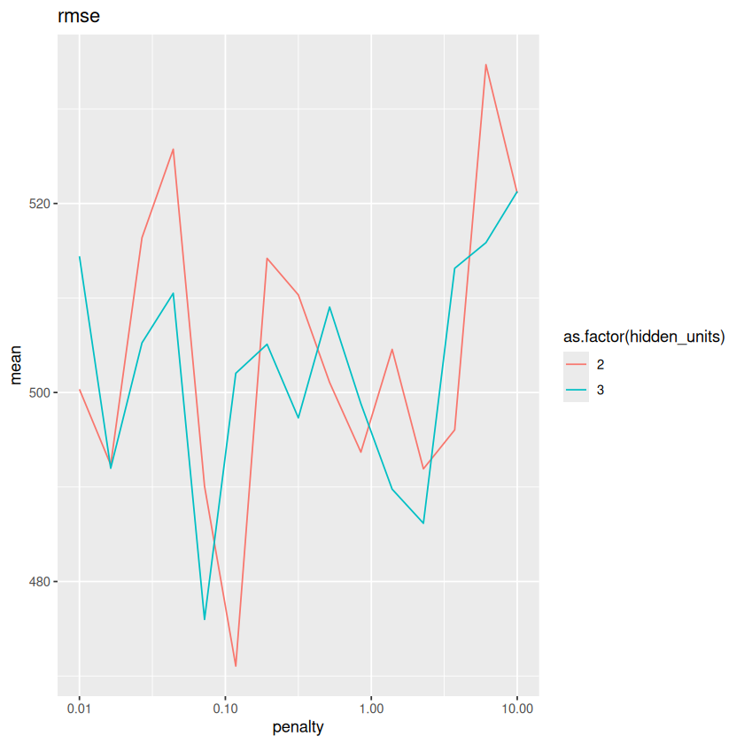
../_images/fa6aa2d1bc9191ffa4a99e1f4c87a48f9f99aef9d31b28de4b9c58adfba15675.png

../_images/f13d110a8f514bc9ac39c6a7fb3212b02fbbbba532c442878cc1360bb6cc48ff.png

The results are very close to each other. What if we add \(std\_err\) as error bars?

for(metric in unique(METRICS$.metric)){
    metrics <- METRICS %>% filter(.metric==metric)
    plot <- ggplot(metrics, aes(x=penalty, y=mean, color=as.factor(hidden_units))) + geom_line() + scale_x_log10() + labs(title=metric)
    plot <- plot + geom_errorbar(aes(ymin=mean-std_err, ymax=mean+std_err))
    print(plot)
}

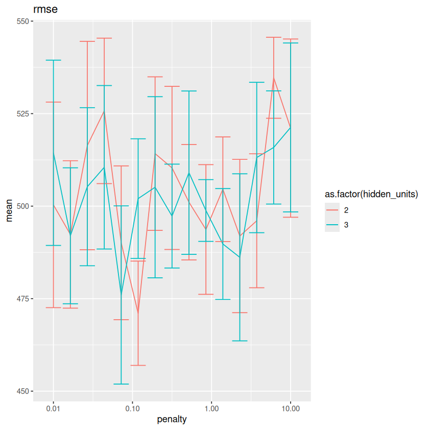
../_images/6e7b9cfa25df19d585922d56cbbbe38fdee8a8e5439261ae2ab9b231dc761128.png

../_images/e9ecad924ebcbc1fc44fa7fc3b0c270e865091ec9e6b538a0947d17cc1a00a80.png

The error bars show that indeed the different models have very similar performances on this particular data. In the following, we still select the best model, but technically others are expected to work as well as the selected one.

BEST <- select_best(RES, metric = 'rmse')
BEST

A tibble: 1 × 3
hidden_units	penalty	.config
<dbl>	<dbl>	<chr>
2	0.1178769	Preprocessor1_Model11

MODEL <- WF %>%
    finalize_workflow(BEST) %>%
    fit(TRAIN)
MODEL

══ Workflow [trained] ══════════════════════════════════════════════════════════════════════════════════════════════════════════════════════════════════════════════════════════════════════════════════════════════
Preprocessor: Recipe
Model: mlp()

── Preprocessor ────────────────────────────────────────────────────────────────────────────────────────────────────────────────────────────────────────────────────────────────────────────────────────────────────
5 Recipe Steps

• step_normalize()
• step_dummy()
• step_nzv()
• step_corr()
• step_lincomb()

── Model ───────────────────────────────────────────────────────────────────────────────────────────────────────────────────────────────────────────────────────────────────────────────────────────────────────────
a 14-2-1 network with 33 weights
inputs: Gestation MotherAge MotherHeight MotherWeight FatherAge FatherHeight FatherWeight MotherEducation_College MotherEducation_HS FatherRace_Black FatherRace_White Father_Education_College Father_Education_HS Smoking_now 
output(s): ..y 
options were - linear output units  decay=0.1178769

Pros and Cons#

Pros:

Can learn nonlinear relationships and create relevant predictors automatically through the use of hidden layers.
Does well when distributions resemble a Normal (symmetric, bell-shaped) curve (many image, text, or speech based problems that humans do) as long as there is a lot of data.
Once trained, predictions are very fast.
Deep learning, which are massive neural networks, actually are amazingly effective at what they are tuned to do.

Cons:

Overhyped early in its history and now. Neural networks will not solve every problem ever created.
Often doesn’t work the best for business problems where distributions do not resemble a Normal curve.
Hard to interpret (like most other models).
Computationally intensive to train and tune (like most other good models).
Well-known for neural network researchers: A neural network is the second best way to solve any problem. The best way is to actually understand the problem.