library(tidymodels)
library(e1071)
library(MASS)
library(ISLR)
library(robustbase)
Show code cell output
── Attaching packages ────────────────────────────────────────────────────────────────────────────────────────────────────────────────────────────────────────────────────────────────────────── tidymodels 1.3.0 ──
✔ broom        1.0.7     ✔ recipes      1.1.1
✔ dials        1.4.0     ✔ rsample      1.2.1
✔ dplyr        1.1.4     ✔ tibble       3.2.1
✔ ggplot2      3.5.1     ✔ tidyr        1.3.1
✔ infer        1.0.7     ✔ tune         1.3.0
✔ modeldata    1.4.0     ✔ workflows    1.2.0
✔ parsnip      1.3.0     ✔ workflowsets 1.1.0
✔ purrr        1.0.4     ✔ yardstick    1.3.2
── Conflicts ───────────────────────────────────────────────────────────────────────────────────────────────────────────────────────────────────────────────────────────────────────────── tidymodels_conflicts() ──
✖ purrr::%||%()    masks base::%||%()
✖ purrr::discard() masks scales::discard()
✖ dplyr::filter()  masks stats::filter()
✖ dplyr::lag()     masks stats::lag()
✖ recipes::step()  masks stats::step()
Attaching package: ‘e1071’
The following object is masked from ‘package:tune’:

    tune
The following object is masked from ‘package:rsample’:

    permutations
The following object is masked from ‘package:parsnip’:

    tune
Attaching package: ‘MASS’
The following object is masked from ‘package:dplyr’:

    select
Support Vector Machines#
Support Vector Machines (SVM) are a relatively recent approach for classification and regression that work well with little user input or tuning (like random forests).
Contrary to the name, the technique has nothing to do with machines. The word “support” applies only in a way mathematicians think. The word “vector” has nothing to do with the vectors we create in R. But it sure sounds fancy.
With classification, the technique is concerned with finding pivotal individuals in the dataset that seem to play a key role in differentiating one class from another. With regression, the technique is concerned with finding pivotal individuals in the dataset to whose errors are important to minimize.
Maximum Margin Classifier#
A separating hyperplane is simply a ``flat” boundary that separates the data space (all possible combinations of the predictor variables) into two regions.
Maybe there’s a separating hyperplane that can evenly split the data space so all individuals on one class are on one side and all members of the other class are on the other side?
With one predictor, the “data space” is just the number line, so a “separating hyperplane” would just be some particular point on the line (or perhaps a “line” that extends into a second dimension (“no man’s land”; a region outside the data space).
Show code cell source
set.seed(474); x <- runif(20,1,3)
y <- rep(0,length(x))
plot(y~x,ylim=c(-.5,.5),col=ifelse(x<1.8,"red","blue"),pch=20,cex=1.4,axes=FALSE,ylab="",xlim=c(1,3))
abline(v=1.78,lwd=2)
abline(h=0)
axis(1,at=seq(1,3,by=0.5))

With two predictors, the data space is visualized as the standard scatterplot, and a “separating hyperplane” would be a line that bisects it. You can imagine this line extending out towards you and away from you into a third dimension (“no man’s land”; not part of the data space).
Show code cell source
set.seed(474); x1 <- runif(30,1,3); x2 <- runif(30,3,5)
plot(x1~x2,col=ifelse(x1+x2<6,"red","blue"),pch=20,cex=1.3)
lines(c(3,5),c(3,1))
With four or more predictor variables, the dataspace is 4-dimensional, and the separating hyperplane would extend into an ``unseen” 5-th dimension. No way to visualize this, but you get the idea.
Note
The maximum margin classifier seeks to find the separating hyperplane that puts the most distance between the nearest example of each class (assuming of course, that it is possible to do so).
Separating Hyperplane#
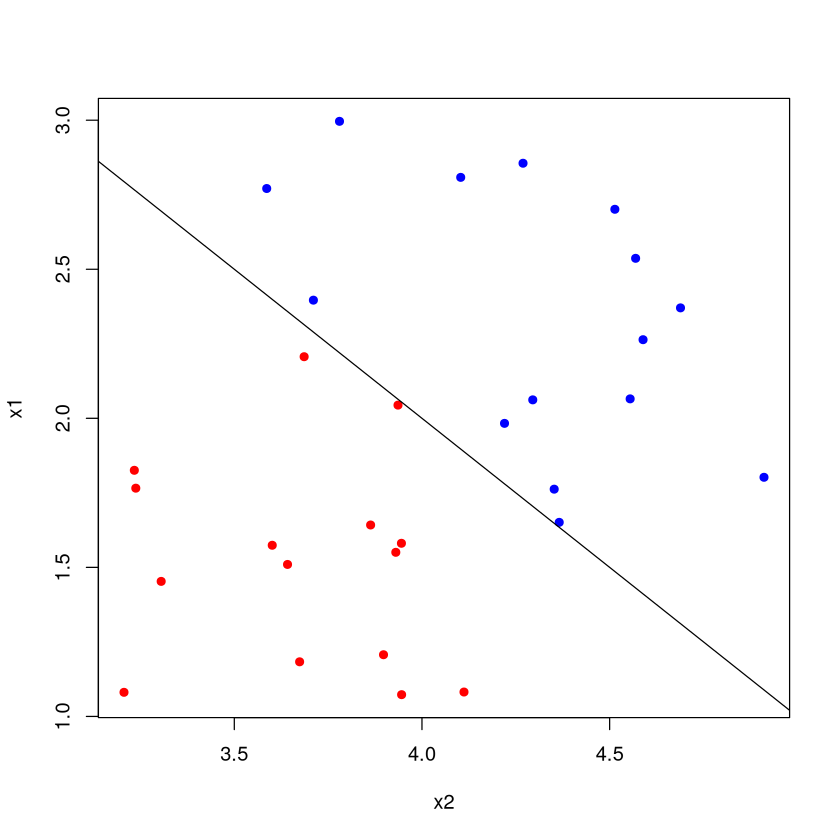
All four of these “separating hyperplanes” succeed in bisecting the data space into a “blue region” and a “red region”. Classification proceeds by figuring out which side a new individual is on: red or blue? But which of these separating hyperplanes is the “best”?
Show code cell source
set.seed(474)
X <- matrix( rnorm(80,.2,.15),ncol=2 )
Y <- matrix( rnorm(80,.73,.17),ncol=2 )
DATA <- as.data.frame( rbind(X,Y) )
names(DATA) <- c("x1","x2")
DATA$class <- factor( c(rep("red",40),rep("blue",40) ))
plot(x2~x1,data=DATA,col=2*as.numeric(DATA$class),pch=20,cex=2)
abline(1,-1.5)
abline(0.9,-1.4)
abline(0.8,-1.2)
abline(3,-6)

Maximal Soft Margin Classifiers#
The maximal margin classifier takes the best separating hyperplane to be the one that gives the largest ``margin” (i.e., spacing; black arrows) between it and the nearest point of each class (on the plot, the distance from the separating hyperplane to the dotted lines measured perpendicularly). All points are not only on the correct side of the hyperplane, \uline{they are also on the correct side of the margin} (red points are above the dashed red line; blue points are below the dashed blue line)!
Show code cell source
set.seed(474)
X <- matrix( rnorm(80,.2,.15),ncol=2 )
Y <- matrix( rnorm(80,.73,.17),ncol=2 )
DATA <- as.data.frame( rbind(X,Y) )
names(DATA) <- c("x1","x2")
DATA$class <- factor( c(rep("red",40),rep("blue",40) ))
DATA <- as.data.frame( rbind(X,Y) )
names(DATA) <- c("x1","x2")
DATA$class <- factor( c(rep("red",40),rep("blue",40) ))
plot(x2~x1,data=DATA,col=2*as.numeric(DATA$class),pch=20,cex=2)
SVM <- svm(class~.,data=DATA,type='C-classification', kernel='linear',scale=FALSE,cost=1000)
W <- t(SVM$coefs) %*% SVM$SV
abline(SVM$rho/W[2],-W[1]/W[2],lwd=3 )
#points(SVM$SV,pch=8,cex=2)
margin <- mean( abs( (SVM$SV)[,2] - SVM$rho/W[2] + W[1]/W[2]*(SVM$SV)[,1]) )
abline(SVM$rho/W[2]+margin,-W[1]/W[2],lty=3,col="blue",lwd=2 )
abline(SVM$rho/W[2]-margin,-W[1]/W[2],lty=3,col="red",lwd=2 )
arrows(-0.01067408,0.4691493,0.14137917,0.8686653,col="blue",lwd=3)
arrows(0.7782815,0.4236349,0.6204904,-0.01128126,col="red",lwd=3)
arrows(0.1700685,0.5247781,0.2618742,0.7270647,col="black",lwd=2,code=3,length=.1)

Support Vectors#
You’ll note that three of the points have been starred. These are the support vectors. They ``support” the separating hyperplane because if their values changed, so would the hyperplane.
Notice that the rest of the data is essentially irrelevant at this point: it’s only the positions of the support vectors that matter. This means the procedure can be quite robust to outliers.
Show code cell source
DATA <- as.data.frame( rbind(X,Y) )
names(DATA) <- c("x1","x2")
DATA$class <- factor( c(rep("red",40),rep("blue",40) ))
plot(x2~x1,data=DATA,col=2*as.numeric(DATA$class),pch=20,cex=2)
SVM <- svm(class~.,data=DATA,type='C-classification', kernel='linear',scale=FALSE,cost=1000)
W <- t(SVM$coefs) %*% SVM$SV
abline(SVM$rho/W[2],-W[1]/W[2],lwd=3 )
points(SVM$SV,pch=8,cex=2)
margin <- mean( abs( (SVM$SV)[,2] - SVM$rho/W[2] + W[1]/W[2]*(SVM$SV)[,1]) )
abline(SVM$rho/W[2]+margin,-W[1]/W[2],lty=3 )
abline(SVM$rho/W[2]-margin,-W[1]/W[2],lty=3 )

What if not separable?#
What if a hyperplane doesn’t neatly divide the data space in two so that all of one class lives on one side and all of the other is on the other side?
Show code cell source
set.seed(474)
X <- matrix( rnorm(80,.2,.15),ncol=2 )
Y <- matrix( rnorm(80,.5,.17),ncol=2 )
DATA <- as.data.frame( rbind(X,Y) )
names(DATA) <- c("x1","x2")
DATA$class <- factor( c(rep("red",40),rep("blue",40) ))
plot(x2~x1,data=DATA,col=2*as.numeric(DATA$class),pch=20,cex=2)

What if a hyperplane doesn’t neatly divide the data space in two so that all of one class lives on one side and all of the other is on the other side?
Support vector classifiers (aka soft margin classifier) allow some observations to be on the wrong side of the margin and even on the wrong side of the hyperplane.
Show code cell source
  set.seed(474)
  X <- matrix( rnorm(80,.2,.15),ncol=2 )
  Y <- matrix( rnorm(80,.5,.17),ncol=2 )
  DATA <- as.data.frame( rbind(X,Y) )
  names(DATA) <- c("x1","x2")
  DATA$class <- factor( c(rep("red",40),rep("blue",40) ))
  plot(x2~x1,data=DATA,col=2*as.numeric(DATA$class),cex=2)

DATA <- as.data.frame( rbind(X,Y) )
names(DATA) <- c("x1","x2")
DATA$class <- factor( c(rep("red",40),rep("blue",40) ))
#plot(x2~x1,data=DATA,col=2*as.numeric(DATA$class),cex=1.5)
SVM <- svm(class~.,data=DATA,type='C-classification', kernel='linear',scale=FALSE,cost=10)
W <- t(SVM$coefs) %*% SVM$SV
abline(SVM$rho/W[2],-W[1]/W[2],lwd=3 )

points(SVM$SV,pch=20,cex=2,col=as.character(DATA$class[ as.numeric(rownames( SVM$SV ) ) ]) )
margin <- max( abs( (SVM$SV)[,2] - SVM$rho/W[2] + W[1]/W[2]*(SVM$SV)[,1]) )
abline(SVM$rho/W[2]+margin,-W[1]/W[2],lty=3,col="blue",lwd=2 )
abline(SVM$rho/W[2]-margin,-W[1]/W[2],lty=3,col="red",lwd=2 )
arrows(-0.05221021,0.2874830,0.07263393,0.7178204,col="blue",lwd=2)
arrows(0.7569648,0.4267098,0.6321207,-0.1091025,col="red",lwd=2)

Soft margin classifier details#
The soft margin classifier depends on a parameter \(C\). This is essentially a ``budget” that allows for some misclassifications.
When \(C>0\), no more than \(C\) observations can be on the wrong side of the hyperplane.
Larger values of \(C\) allow more misclassifications (and more support vectors).
Smaller values of \(C\) allow fewer misclassifications (and fewer support vectors).
The ``best” value of \(C\) is typically estimated with cross-validation, since its value will depend on how mixed together the classes are. Smaller values of \(C\) yield models that are more complex and fit the training data better (since few misclassifications are allowed). Larger values of \(C\) yield simpler models which may generalize better (at the cost of less accuracy).
Kernel Trick in Support Vector Machine#
Pictured is an extreme artificial case where no hyperplane would do a good job separating the classes, but there is still a distinct but nonlinear boundary.
Show code cell source
set.seed(474)
plot(0,0,col="white",xlim=c(-1,1),ylim=c(-1,1),xlab="x1",ylab="x2")
INNER <- matrix(0,ncol=2,nrow=150)
OUTER <- INNER
i <- 1
while( i <= 150 ) {
  x <- runif(2,-1,1)
  if( x[1]^2 + x[2]^2 <= .5^2 ) { INNER[i,] <- x; i <- i+ 1}
}
i<-1
while( i <= 150 ) {
  x <- runif(2,-1,1)
  if( x[1]^2 + x[2]^2 <= 1 & x[1]^2 + x[2]^2 >= .5^2 ) { OUTER[i,] <- x; i <- i+ 1}
}
points(INNER,cex=1,pch=20,col="red")
points(OUTER,cex=1,pch=20,col="blue")

Support vector machines are somewhat unique in the field of data mining and machine learning in that it takes the philosophy that the model is good, it’s the data that needs to become more flexible.
The support vector machine believes that a linear regression (for numerical \(y\)) is a great model, it’s just that the original data space isn’t the place to fit it. Likewise, it believes that a flat boundary (separating hyperplane) is a great way to make classifications, it’s just the original data space isn’t the place to use it.
This is in stark contrast to other models that that the observed values (or transformations or derived quantities) as is, then modifies the model until there’s a good fit.
The support vector machine is an extension to the soft margin classifier that uses the ``kernel trick” to discern non-linear boundaries between classes.
The mathematics of the kernel trick are beyond the scope of this course, but in essence it takes the original data and projects it into a data space of higher dimensionality, where it hopes it can find a separating hyperplane.
Usually, the ``curse of dimensionality” means that tasks in high dimensions (many predictors) become difficult. It just so happens to be the case that sometimes it makes tasks easier.
Kernel Trick#
Imagine classifying individuals as red or blue depending on the value of their value of \(x\). It is clear that no separating hyperplane exists. It is also clear that a non-linear boundary exists between the two classes. However, this ``boundary” reaches outside the dataspace (the one-dimensional line).
Show code cell source
plot(0,0,col="white",xlab="x",ylab="",xlim=c(0,1),ylim=c(-.5,.5),yaxt='n')
abline(h=0)
set.seed(474)
x <- runif(30)
x[1:2] <- c(.38,.52)
y <- factor( ifelse(x < 0.6 & x >0.37,"red","blue") )
points(x,rep(0,length(x)),col=as.character(y),pch=20,cex=1.5)
curve( 10*(x-0.35)*(x-0.55), add=TRUE )

The problem is that figuring out a non-linear boundary is very difficult because there are so many possible shapes it could take. Lines and hyperplanes are much easier to work with, so instead of trying to figure out the non-linear boundary, the ``kernel trick” takes the data and projects it into a higher dimensional space where it hopes a separating hyperplane exists.
What does ``projecting into a higher dimensional space” even mean? It basically means creating new variables from ones that you already have. If \(x\) is the one predictor you have collected, then using \(x^2\) and \(\log x\) as additional predictors essentially makes the data space have three dimensions.
These ``new” predictors don’t contain any new information about the classes of course, but oddly enough, they can make the boundary between classes linear.
Project from one to two dimensions#
There was no separating hyperplane in the 1D dataspace (just \(x\) as a predictor). But by projecting into a 2D database by adding \(x^2\) as a predictor, all of a sudden there is a separating hyperplane.
Show code cell source
plot(x,x^2,col=as.character(y),xlab="x",ylab="square of x",xlim=c(0,1),pch=20)
m <- (.52^2-.38^2)/(.52-.38)
b <- .38^2 - m*.38
abline(b+.005,m)

Projecting from two to three dimensions#
There is no separating hyperplane in the 2D dataspace using the predictors \(x_1\) and \(x_2\). But we do see that a curved boundary exists.
Show code cell source
set.seed(474)
plot(0,0,col="white",xlim=c(-1,1),ylim=c(-1,1),xlab="x1",ylab="x2")
INNER <- matrix(0,ncol=2,nrow=150)
OUTER <- INNER
i <- 1
while( i <= 150 ) {
  x <- runif(2,-1,1)
  if( x[1]^2 + x[2]^2 <= .48^2 ) { INNER[i,] <- x; i <- i+ 1}
}
i<-1
while( i <= 150 ) {
  x <- runif(2,-1,1)
  if( x[1]^2 + x[2]^2 <= 1 & x[1]^2 + x[2]^2 >= .52^2 ) { OUTER[i,] <- x; i <- i+ 1}
}
points(INNER,col="red")
points(OUTER,col="blue")

Projecting from two to three dimensions#
By adding a third “predictor” \(x_3 = x_1^2 + x_2^2\) (no new information about the problem), the data space becomes 3D. Now there is a separating hyperplane that neatly divides the space into a “red region” and “blue region”, achieving 100% accuracy.
Show code cell source
DATA <- data.frame(x1=rbind(INNER,OUTER)[,1],x2=rbind(INNER,OUTER)[,2])
DATA$x3 <- DATA$x1^2 + DATA$x2^2
plot(0,0,col="white",xlim=c(-1,1),ylim=c(0,1),xlab="x1",ylab="x3")
points(DATA[,c('x1','x3')],col=c(rep("red",150),rep("blue",150)))

Adding additional predictors to project the data into a higher dimensional space often works, but the question is: what predictors? There’s an infinite number of possible combinations.
SVMs use the ``kernel trick” to get around this problem. A kernel is just a matrix whose values record a somewhat abstract measure of similarity (kind of like a distance) between individuals. The values of the kernel matrix are given by an equation we choose, like
The amazing thing is that by defining the kernel matrix, we can implicitly define additional predictors without specifying exactly what they are or how to get them.
Kernels#
Note
It turns out that the equation for the optimal separating hyperplane does not depend on the exact locations (coordinates) of the individuals in the higher-dimension space we are projecting into. Rather, it depends only the entries in the kernel matrix, i.e., how we quantify the similarity between two individuals.
Don’t actually have to project each individual into the higher dimensional space, only have to compute kernel/similarities (more computationally efficient).
Kernel implicitly captures the higher-dimensional space without explicitly having to construct it. This allows projecting into infinite dimensional spaces when exploring the existence of a separating hyperplane.
This is all very trippy stuff!
If you are pressed for a simple explanation, try out the following oversimplification.
Note
When doing classification, support vector machines assigns a score to each individual, where the score is some number derived from transformations of the predictor variables. If that score exceeds a certain threshold, it is assigned class A. Otherwise it is assigned class B.
Popular kernels#
Let the predictor variables are \(a\), \(b\), \(c\), etc., then the inner product between individuals \(i\) and \(j\) is the sum of the products of the individuals’ predictor variables.
Linear (this is just the soft margin classifier, good for when boundary between classes is hyperplane in the recorded variables):
Polynomial of order \(d\) (good for when boundary between classes is a curve that can be captured by some polynomial in the recorded variables):
Radial basis or Gaussian (general purpose; only ``nearby” training observations have an impact on how a new individual is classified):
Radial Basis Kernel#
Like ``magic”, the SVM with a radial basis kernel is able to recognize that the boundary between classes is non-linear, and does a pretty good job at figuring it out. The circles in this plot represent correct classifications and the X’s represent misclassifications.
Show code cell source
DATA <- as.data.frame( rbind(INNER,OUTER) )
names(DATA) <- c("x1","x2")
DATA$y <- factor( c(rep("red",150),rep("blue",150)))
plot(DATA[,2:1],col=as.character(DATA[,3]),pch=20)
SVM <- svm(y~.,data=DATA,type='C-classification', kernel='radial',scale=FALSE,cost=50)
plot(SVM,DATA)


Another example.
Show code cell source
DATA <- as.data.frame(matrix(runif(300,-1,1),ncol=2))
DATA[,2] <- DATA[,2]+.5
names(DATA) <- c("x1","x2")
DATA$y <- factor( ifelse(DATA[,2] > DATA[,1]^2,"red","blue"))
plot(DATA[,2:1],col=as.character(DATA[,3]),pch=20)
curve(sqrt(abs(pmax(0,x))),add=TRUE,n=1001,from=-.01,to=1.7)
curve(-sqrt(abs(pmax(0,x))),add=TRUE,n=1001,from=-.01,to=1.7)
SVM <- svm(y~.,data=DATA,type='C-classification', kernel='radial',scale=FALSE,cost=15)
plot(SVM,DATA)


Support Vector Machines for classification summary#
While the whole procedure seems a bit wild and too good to be true, SVMs often work well in practice. The two main considerations are:
What kernel to use? Popular choices are the polynomial kernel (new predictors are polynomial combinations of the original ones) and the radial basis kernel / Gaussian kernel (which projects into the infinite dimensional space by essentially using an infinite number of polynomials).
What parameters of the kernel should be used? Polynomial needs a “degree” parameter (how many powers of the predictors should be used). The radial basis kernel needs a “spread” parameter (\(gamma\)) which controls how quickly the values inside the kernel matrix decrease with the distance between individuals.
What is the ``cost parameter”, i.e., the penalty to apply to a proposed separating hyperplane when it makes misclassifications. Larger costs make the model fit the training data better (lower bias) at the expense of increasing its variance (sensitivity to the training data) and its risk of overfitting.
Support Vector Machines (SVM) approaches classification in a new and interesting way.
Find a ``separating hyperplane” (basically a flat plane) that divides the data space into two parts where most (hopefully all) members of a class are on one side of the plane.
The location of this separating hyperplane is dependent on only a few pivotal individuals in the dataset (the support vectors) so the solution is ``sparse”. With fewer features, the prediction algorithm is extremely memory and computationally efficient (once the model is fit).
Problem: the boundary between classes may not be well-described by a straight edge!
Solution: project the data into a higher-dimensional data space (i.e., create new variables from the ones where we already have) where the boundary is better described by a straight edge.
Support Vector Machines for Regression#
Support Vector Machines can also be used to predict numerical responses (just ``won” a class competition in BAS 479). The procedure borrows heavily from that used for classification.
SVM assumes that there is a linear relationship between the \(y\) variable and some predictor variables (the \(x\)’s). However, these predictors may not be the raw values that have been collected.
We will project the data into a higher dimensional data space with the “kernel trick”, thereby implicitly creating new predictor variables. With the “right” kernel, relationships may be approximately linear.
A linear regression model is fit to the relationship in this higher-dimensional space but with a twist: not all errors made by the model count against it.
Instead of choosing the form of the linear regression by minimizing its sum of squared errors, we will minimize the sum of absolute values of only errors that are ``large” (greater than some threshold).
The support vectors will be the points whose errors contributed to the form of the model, so once again the model is ``sparse” (depends only on a few pivotal individuals).
How it works#
The errors (lines connecting the dots to the solid blue line) ``don’t count” if they are smaller than some threshold \(\epsilon\) (thick vertical black line segment). \uline{SVM finds the line whose coefficients are closest to 0 (i.e., regularization is being performed) and whose errors (specifically errors in excess of \(\epsilon\), given by the length of the red segments) are smallest}. The support vectors (stars) are the points whose errors are in excess of \(\epsilon\).
Show code cell source
set.seed(479)
x <- seq(2,10,length=10)
y <- 5*x + 20 + rnorm(length(x),0,10)
plot(y~x,pch=20,cex=1.5,xlim=c(1,11),ylim=c(10,90))
M <- lm(y~x)
abline(lsfit(x,y),col="blue",lwd=2)
slope <- coef(lm(y~x))[2]
intercept <- coef(M)[1]
abline(intercept-10,slope,lty=2,col="blue")
abline(intercept+10,slope,lty=2,col="blue")
for(i in 1:10) { lines( c(x[i],x[i]), c(y[i],fitted(M)[i]),col=ifelse( abs(y[i]-fitted(M)[i]) > 10,"green","green"  ),lwd=ifelse( abs(y[i]-fitted(M)[i]) > 10,2,1 ),lty=1   ) }
lines( c(6.7,6.7), c( predict(M,newdata=data.frame(x=6.7)), predict(M,newdata=data.frame(x=6.7))+10 ),lwd=4)
text(6.5,63,expression(epsilon),cex=1.5)
oops <- which( abs( fitted(M) - y ) > 10 )
for (i in oops) {
  lines(  c(x[i],x[i]), c(y[i],fitted(M)[i] + 10*ifelse(y[i]>fitted(M)[i],1,-1)  ) ,col="red",lwd=3 )
}
points(x,y,pch=ifelse( abs(y-fitted(M))>10,8,1),cex=1.2)

Bias-variance tradeoff#
When the form of the SVM is being determined, it balances the bias and variance of the resulting model through the use of a cost parameter \(C\).
Large values of \(C\) focus the attention towards the errors made by the model. The result will be a model that has a low bias (it fits the training data well) but potentially high variance (poor generalizability due to sensitivity to the specific individuals in the training data).
Small values of \(C\) focus the attention towards the size of the coefficients. The result will be a model that makes a larger error on the training data (higher bias since it won’t have as much ``wiggle room” to fit the data) but that has a lower variance (not as sensitive to the individuals in the data).
The optimal value of the cost parameter \(C\), the error threshold \(\epsilon\), and any kernel specific parameters (the degree in a polynomial kernel and the ``gamma” parameter of a radial basis kernel) is found via cross-validation.
Larger cost = errors are weighted more. Model will fit the data better, but could be too wiggly to generalize.
Lower cost = coefficients are weighted more. Model will not be as wiggly and will have a larger error on the training, but at least it is not overfit.
Show code cell source
set.seed(474)
x <- sort( runif(50,2,10) )
y <- x^2*sin(x) + 200 + rnorm(50,0,10)
plot(y~x,pch=20,cex=1.5)
SVM <- svm(x,y,scale=TRUE,cost=.1)
new <- data.frame(x=seq(2,10,length=500) )
pred.y <- predict(SVM,newdata=new,scale=TRUE)
lines(new$x,pred.y,col="black")
SVM <- svm(x,y,scale=TRUE,cost=10)
new <- data.frame(x=seq(2,10,length=500) )
pred.y <- predict(SVM,newdata=new,scale=TRUE)
lines(new$x,pred.y,col="red")
legend("topleft",c("Cost=0.1","Cost=10"),lty=1,col=c("black","red"))

Tuning parameters and making predictions#
Tuning the parameters in \(e1071\)#
The \(e1071\) package offers an additional options that are not available through \(train\) and \(caret\) that you should be aware of. The cost and \(\epsilon\) (epsilon) parameters always must be tuned. The default kernel is the radial basis kernel, and this requires additional tuning of the ``gamma” parameter (how quickly the entries of the kernel matrix go to 0 for points that are separated by larger distances). It’s possible to use \(tune\) from the \(e1071\) library.
# perform a grid search
SVMparams <- tune("svm", y~x,ranges=
                    list(epsilon=seq(0,1,0.2),cost=2^(2:8),gamma=10^(seq(-3,1,.5))))
SVMparams
Parameter tuning of ‘svm’:

- sampling method: 10-fold cross validation

- best parameters:
 epsilon cost     gamma
     0.2  256 0.3162278

- best performance: 79.12614
Plotting the selected model#
In this case, the defaults do a pretty good job (at least visually), but the selected parameters are designed to offer a reasonable tradeoff between the bias and complexity of the model so that it generalizes well to new data.
plot(y~x,pch=20,cex=1.5)
SVM <- svm(x,y,scale=TRUE,cost=256,gamma=0.3162278,epsilon=0.2)
new <- data.frame(x=seq(2,10,length=500) )
pred.y <- predict(SVM,newdata=new,scale=TRUE)
lines(new$x,pred.y,col="red")

Support vector machines with tidymodels#
Now we build SVMs with tidymodels. We try both linear and non-linear kernels:
svm_linear() defines a support vector machine model. For classification, the model tries to maximize the width of the margin between classes (using a linear class boundary). For regression, the model optimizes a robust loss function that is only affected by very large model residuals and uses a linear fit.
svm_poly() defines a support vector machine model. For classification, the model tries to maximize the width of the margin between classes using a polynomial class boundary. For regression, the model optimizes a robust loss function that is only affected by very large model residuals and uses polynomial functions of the predictors.
svm_rbf() defines a support vector machine model. For classification, the model tries to maximize the width of the margin between classes using a nonlinear class boundary. For regression, the model optimizes a robust loss function that is only affected by very large model residuals and uses nonlinear functions of the predictors.
An example with regression problem.#
data(BODYFAT, package='regclass')

# This is not usually right if want to investigate testing performances.
TRAIN <- BODYFAT

REC <- recipe(BodyFat ~ ., TRAIN) %>%
    step_normalize(all_numeric_predictors()) %>%
    step_dummy(all_nominal_predictors()) %>%
    step_nzv(all_predictors()) %>%
    step_corr(all_predictors()) %>%
    step_lincomb(all_predictors())

WF <- workflow() %>%
    add_recipe(REC) %>%
    add_model(svm_linear( mode = 'regression', cost = tune() ))

GRID <- expand.grid( cost = 10^seq(-1,2,by=0.5) )

RES <- WF %>%
    tune_grid(
        resamples = vfold_cv(TRAIN, v = 5),
        grid = GRID,
    )

METRICS <- collect_metrics(RES)

METRICS
| cost | .metric | .estimator | mean | n | std_err | .config |
|---|---|---|---|---|---|---|
| <dbl> | <chr> | <chr> | <dbl> | <int> | <dbl> | <chr> |
| 0.1000000 | rmse | standard | 4.2334779 | 5 | 0.19911762 | Preprocessor1_Model1 |
| 0.1000000 | rsq | standard | 0.7075926 | 5 | 0.01175335 | Preprocessor1_Model1 |
| 0.3162278 | rmse | standard | 4.2334779 | 5 | 0.19911762 | Preprocessor1_Model2 |
| 0.3162278 | rsq | standard | 0.7075926 | 5 | 0.01175335 | Preprocessor1_Model2 |
| 1.0000000 | rmse | standard | 4.2334779 | 5 | 0.19911762 | Preprocessor1_Model3 |
| 1.0000000 | rsq | standard | 0.7075926 | 5 | 0.01175335 | Preprocessor1_Model3 |
| 3.1622777 | rmse | standard | 4.2334779 | 5 | 0.19911762 | Preprocessor1_Model4 |
| 3.1622777 | rsq | standard | 0.7075926 | 5 | 0.01175335 | Preprocessor1_Model4 |
| 10.0000000 | rmse | standard | 4.2334779 | 5 | 0.19911762 | Preprocessor1_Model5 |
| 10.0000000 | rsq | standard | 0.7075926 | 5 | 0.01175335 | Preprocessor1_Model5 |
| 31.6227766 | rmse | standard | 4.2334779 | 5 | 0.19911762 | Preprocessor1_Model6 |
| 31.6227766 | rsq | standard | 0.7075926 | 5 | 0.01175335 | Preprocessor1_Model6 |
| 100.0000000 | rmse | standard | 4.2334779 | 5 | 0.19911762 | Preprocessor1_Model7 |
| 100.0000000 | rsq | standard | 0.7075926 | 5 | 0.01175335 | Preprocessor1_Model7 |
WF <- workflow() %>%
    add_recipe(REC) %>%
    add_model(svm_poly( mode = 'regression', cost = tune(), degree = tune() ))

GRID <- expand.grid( cost = 10^seq(-1,2,by=0.5), degree = seq(1,3) )

RES <- WF %>%
    tune_grid(
        resamples = vfold_cv(TRAIN, v = 5),
        grid = GRID,
    )

METRICS <- collect_metrics(RES)

METRICS
| cost | degree | .metric | .estimator | mean | n | std_err | .config |
|---|---|---|---|---|---|---|---|
| <dbl> | <int> | <chr> | <chr> | <dbl> | <int> | <dbl> | <chr> |
| 0.1000000 | 1 | rmse | standard | 4.2772574 | 5 | 0.05810841 | Preprocessor1_Model01 |
| 0.1000000 | 1 | rsq | standard | 0.6884937 | 5 | 0.03654208 | Preprocessor1_Model01 |
| 0.3162278 | 1 | rmse | standard | 4.2528116 | 5 | 0.06796573 | Preprocessor1_Model02 |
| 0.3162278 | 1 | rsq | standard | 0.6907363 | 5 | 0.04110505 | Preprocessor1_Model02 |
| 1.0000000 | 1 | rmse | standard | 4.2453571 | 5 | 0.07287966 | Preprocessor1_Model03 |
| 1.0000000 | 1 | rsq | standard | 0.6919614 | 5 | 0.03914640 | Preprocessor1_Model03 |
| 3.1622777 | 1 | rmse | standard | 4.2320469 | 5 | 0.07855867 | Preprocessor1_Model04 |
| 3.1622777 | 1 | rsq | standard | 0.6932687 | 5 | 0.03972725 | Preprocessor1_Model04 |
| 10.0000000 | 1 | rmse | standard | 4.2358162 | 5 | 0.07803618 | Preprocessor1_Model05 |
| 10.0000000 | 1 | rsq | standard | 0.6929180 | 5 | 0.03957301 | Preprocessor1_Model05 |
| 31.6227766 | 1 | rmse | standard | 4.2366662 | 5 | 0.07725952 | Preprocessor1_Model06 |
| 31.6227766 | 1 | rsq | standard | 0.6927763 | 5 | 0.03956189 | Preprocessor1_Model06 |
| 100.0000000 | 1 | rmse | standard | 4.2386710 | 5 | 0.07667949 | Preprocessor1_Model07 |
| 100.0000000 | 1 | rsq | standard | 0.6924852 | 5 | 0.03955387 | Preprocessor1_Model07 |
| 0.1000000 | 2 | rmse | standard | 5.2153421 | 5 | 0.25317917 | Preprocessor1_Model08 |
| 0.1000000 | 2 | rsq | standard | 0.5758829 | 5 | 0.06429783 | Preprocessor1_Model08 |
| 0.3162278 | 2 | rmse | standard | 5.7140481 | 5 | 0.22669922 | Preprocessor1_Model09 |
| 0.3162278 | 2 | rsq | standard | 0.5296920 | 5 | 0.06855940 | Preprocessor1_Model09 |
| 1.0000000 | 2 | rmse | standard | 7.5380347 | 5 | 1.03636336 | Preprocessor1_Model10 |
| 1.0000000 | 2 | rsq | standard | 0.4173636 | 5 | 0.08193462 | Preprocessor1_Model10 |
| 3.1622777 | 2 | rmse | standard | 8.5160534 | 5 | 1.69340525 | Preprocessor1_Model11 |
| 3.1622777 | 2 | rsq | standard | 0.3901460 | 5 | 0.07930041 | Preprocessor1_Model11 |
| 10.0000000 | 2 | rmse | standard | 8.6303556 | 5 | 1.77936173 | Preprocessor1_Model12 |
| 10.0000000 | 2 | rsq | standard | 0.3867060 | 5 | 0.07652065 | Preprocessor1_Model12 |
| 31.6227766 | 2 | rmse | standard | 8.5630588 | 5 | 1.73669920 | Preprocessor1_Model13 |
| 31.6227766 | 2 | rsq | standard | 0.3954085 | 5 | 0.06915727 | Preprocessor1_Model13 |
| 100.0000000 | 2 | rmse | standard | 9.2302374 | 5 | 1.62033764 | Preprocessor1_Model14 |
| 100.0000000 | 2 | rsq | standard | 0.3393308 | 5 | 0.09226738 | Preprocessor1_Model14 |
| 0.1000000 | 3 | rmse | standard | 91.3880946 | 5 | 68.46649436 | Preprocessor1_Model15 |
| 0.1000000 | 3 | rsq | standard | 0.1263342 | 5 | 0.06111487 | Preprocessor1_Model15 |
| 0.3162278 | 3 | rmse | standard | 141.5058503 | 5 | 120.19382589 | Preprocessor1_Model16 |
| 0.3162278 | 3 | rsq | standard | 0.1503114 | 5 | 0.06539197 | Preprocessor1_Model16 |
| 1.0000000 | 3 | rmse | standard | 245.4066103 | 5 | 222.76878794 | Preprocessor1_Model17 |
| 1.0000000 | 3 | rsq | standard | 0.1660929 | 5 | 0.05626166 | Preprocessor1_Model17 |
| 3.1622777 | 3 | rmse | standard | 272.7828149 | 5 | 249.50410098 | Preprocessor1_Model18 |
| 3.1622777 | 3 | rsq | standard | 0.1605847 | 5 | 0.05414295 | Preprocessor1_Model18 |
| 10.0000000 | 3 | rmse | standard | 272.7828149 | 5 | 249.50410098 | Preprocessor1_Model19 |
| 10.0000000 | 3 | rsq | standard | 0.1605847 | 5 | 0.05414295 | Preprocessor1_Model19 |
| 31.6227766 | 3 | rmse | standard | 272.7828149 | 5 | 249.50410098 | Preprocessor1_Model20 |
| 31.6227766 | 3 | rsq | standard | 0.1605847 | 5 | 0.05414295 | Preprocessor1_Model20 |
| 100.0000000 | 3 | rmse | standard | 272.7828149 | 5 | 249.50410098 | Preprocessor1_Model21 |
| 100.0000000 | 3 | rsq | standard | 0.1605847 | 5 | 0.05414295 | Preprocessor1_Model21 |
WF <- workflow() %>%
    add_recipe(REC) %>%
    add_model(svm_rbf( mode = 'regression', cost = tune(), rbf_sigma = tune() ))

GRID <- expand.grid( cost = 10^seq(-1,2,by=0.5), rbf_sigma = 10^seq(-3,0,by=0.5) )

RES <- WF %>%
    tune_grid(
        resamples = vfold_cv(TRAIN, v = 5),
        grid = GRID,
    )

METRICS <- collect_metrics(RES)

METRICS
| cost | rbf_sigma | .metric | .estimator | mean | n | std_err | .config |
|---|---|---|---|---|---|---|---|
| <dbl> | <dbl> | <chr> | <chr> | <dbl> | <int> | <dbl> | <chr> |
| 0.1000000 | 0.001000000 | rmse | standard | 7.2193444 | 5 | 0.380066743 | Preprocessor1_Model01 |
| 0.1000000 | 0.001000000 | rsq | standard | 0.4623490 | 5 | 0.026279555 | Preprocessor1_Model01 |
| 0.3162278 | 0.001000000 | rmse | standard | 6.5169477 | 5 | 0.391014745 | Preprocessor1_Model02 |
| 0.3162278 | 0.001000000 | rsq | standard | 0.4890917 | 5 | 0.028176366 | Preprocessor1_Model02 |
| 1.0000000 | 0.001000000 | rmse | standard | 5.6242385 | 5 | 0.361280294 | Preprocessor1_Model03 |
| 1.0000000 | 0.001000000 | rsq | standard | 0.5648684 | 5 | 0.033165114 | Preprocessor1_Model03 |
| 3.1622777 | 0.001000000 | rmse | standard | 4.8112776 | 5 | 0.319776846 | Preprocessor1_Model04 |
| 3.1622777 | 0.001000000 | rsq | standard | 0.6393887 | 5 | 0.026069230 | Preprocessor1_Model04 |
| 10.0000000 | 0.001000000 | rmse | standard | 4.2812841 | 5 | 0.287633312 | Preprocessor1_Model05 |
| 10.0000000 | 0.001000000 | rsq | standard | 0.6991226 | 5 | 0.021149283 | Preprocessor1_Model05 |
| 31.6227766 | 0.001000000 | rmse | standard | 4.0641470 | 5 | 0.193576958 | Preprocessor1_Model06 |
| 31.6227766 | 0.001000000 | rsq | standard | 0.7244006 | 5 | 0.009198177 | Preprocessor1_Model06 |
| 100.0000000 | 0.001000000 | rmse | standard | 4.0613777 | 5 | 0.126205181 | Preprocessor1_Model07 |
| 100.0000000 | 0.001000000 | rsq | standard | 0.7271831 | 5 | 0.014283924 | Preprocessor1_Model07 |
| 0.1000000 | 0.003162278 | rmse | standard | 6.6063137 | 5 | 0.396994794 | Preprocessor1_Model08 |
| 0.1000000 | 0.003162278 | rsq | standard | 0.4930286 | 5 | 0.023542752 | Preprocessor1_Model08 |
| 0.3162278 | 0.003162278 | rmse | standard | 5.6317618 | 5 | 0.369515614 | Preprocessor1_Model09 |
| 0.3162278 | 0.003162278 | rsq | standard | 0.5651315 | 5 | 0.026921486 | Preprocessor1_Model09 |
| 1.0000000 | 0.003162278 | rmse | standard | 4.7901056 | 5 | 0.307670897 | Preprocessor1_Model10 |
| 1.0000000 | 0.003162278 | rsq | standard | 0.6518101 | 5 | 0.023240692 | Preprocessor1_Model10 |
| 3.1622777 | 0.003162278 | rmse | standard | 4.2562479 | 5 | 0.261801485 | Preprocessor1_Model11 |
| 3.1622777 | 0.003162278 | rsq | standard | 0.7085381 | 5 | 0.017381385 | Preprocessor1_Model11 |
| 10.0000000 | 0.003162278 | rmse | standard | 4.0908816 | 5 | 0.169849564 | Preprocessor1_Model12 |
| 10.0000000 | 0.003162278 | rsq | standard | 0.7225774 | 5 | 0.013465151 | Preprocessor1_Model12 |
| 31.6227766 | 0.003162278 | rmse | standard | 4.0932864 | 5 | 0.106654798 | Preprocessor1_Model13 |
| 31.6227766 | 0.003162278 | rsq | standard | 0.7237566 | 5 | 0.014452649 | Preprocessor1_Model13 |
| 100.0000000 | 0.003162278 | rmse | standard | 4.1531276 | 5 | 0.105710772 | Preprocessor1_Model14 |
| 100.0000000 | 0.003162278 | rsq | standard | 0.7172330 | 5 | 0.011932147 | Preprocessor1_Model14 |
| 0.1000000 | 0.010000000 | rmse | standard | 5.8847100 | 5 | 0.386888762 | Preprocessor1_Model15 |
| 0.1000000 | 0.010000000 | rsq | standard | 0.5476825 | 5 | 0.028620466 | Preprocessor1_Model15 |
| ⋮ | ⋮ | ⋮ | ⋮ | ⋮ | ⋮ | ⋮ | ⋮ |
| 100.0000000 | 0.1000000 | rmse | standard | 6.4155504 | 5 | 0.32635118 | Preprocessor1_Model35 |
| 100.0000000 | 0.1000000 | rsq | standard | 0.4360800 | 5 | 0.07095699 | Preprocessor1_Model35 |
| 0.1000000 | 0.3162278 | rmse | standard | 6.4946261 | 5 | 0.43613805 | Preprocessor1_Model36 |
| 0.1000000 | 0.3162278 | rsq | standard | 0.4736080 | 5 | 0.03708764 | Preprocessor1_Model36 |
| 0.3162278 | 0.3162278 | rmse | standard | 5.6362026 | 5 | 0.43931174 | Preprocessor1_Model37 |
| 0.3162278 | 0.3162278 | rsq | standard | 0.5392246 | 5 | 0.02671818 | Preprocessor1_Model37 |
| 1.0000000 | 0.3162278 | rmse | standard | 5.1931752 | 5 | 0.38012825 | Preprocessor1_Model38 |
| 1.0000000 | 0.3162278 | rsq | standard | 0.5722448 | 5 | 0.01260412 | Preprocessor1_Model38 |
| 3.1622777 | 0.3162278 | rmse | standard | 5.2187727 | 5 | 0.33864221 | Preprocessor1_Model39 |
| 3.1622777 | 0.3162278 | rsq | standard | 0.5569203 | 5 | 0.02404800 | Preprocessor1_Model39 |
| 10.0000000 | 0.3162278 | rmse | standard | 5.2571019 | 5 | 0.32352796 | Preprocessor1_Model40 |
| 10.0000000 | 0.3162278 | rsq | standard | 0.5489426 | 5 | 0.02967668 | Preprocessor1_Model40 |
| 31.6227766 | 0.3162278 | rmse | standard | 5.2571019 | 5 | 0.32352796 | Preprocessor1_Model41 |
| 31.6227766 | 0.3162278 | rsq | standard | 0.5489426 | 5 | 0.02967668 | Preprocessor1_Model41 |
| 100.0000000 | 0.3162278 | rmse | standard | 5.2571019 | 5 | 0.32352796 | Preprocessor1_Model42 |
| 100.0000000 | 0.3162278 | rsq | standard | 0.5489426 | 5 | 0.02967668 | Preprocessor1_Model42 |
| 0.1000000 | 1.0000000 | rmse | standard | 7.5253833 | 5 | 0.38366783 | Preprocessor1_Model43 |
| 0.1000000 | 1.0000000 | rsq | standard | 0.2324882 | 5 | 0.03983346 | Preprocessor1_Model43 |
| 0.3162278 | 1.0000000 | rmse | standard | 7.2473472 | 5 | 0.40711516 | Preprocessor1_Model44 |
| 0.3162278 | 1.0000000 | rsq | standard | 0.2583491 | 5 | 0.03670843 | Preprocessor1_Model44 |
| 1.0000000 | 1.0000000 | rmse | standard | 6.7914166 | 5 | 0.43822868 | Preprocessor1_Model45 |
| 1.0000000 | 1.0000000 | rsq | standard | 0.3313275 | 5 | 0.03799679 | Preprocessor1_Model45 |
| 3.1622777 | 1.0000000 | rmse | standard | 6.6751977 | 5 | 0.44997757 | Preprocessor1_Model46 |
| 3.1622777 | 1.0000000 | rsq | standard | 0.3501769 | 5 | 0.03892751 | Preprocessor1_Model46 |
| 10.0000000 | 1.0000000 | rmse | standard | 6.6751804 | 5 | 0.44997577 | Preprocessor1_Model47 |
| 10.0000000 | 1.0000000 | rsq | standard | 0.3501800 | 5 | 0.03892593 | Preprocessor1_Model47 |
| 31.6227766 | 1.0000000 | rmse | standard | 6.6751804 | 5 | 0.44997577 | Preprocessor1_Model48 |
| 31.6227766 | 1.0000000 | rsq | standard | 0.3501800 | 5 | 0.03892593 | Preprocessor1_Model48 |
| 100.0000000 | 1.0000000 | rmse | standard | 6.6751804 | 5 | 0.44997577 | Preprocessor1_Model49 |
| 100.0000000 | 1.0000000 | rsq | standard | 0.3501800 | 5 | 0.03892593 | Preprocessor1_Model49 |
An example with classification problem.#
data(WINE, package='regclass')

# This is not usually right if want to investigate testing performances.
TRAIN <- WINE

REC <- recipe(Quality ~ ., TRAIN) %>%
    step_normalize(all_numeric_predictors()) %>%
    step_dummy(all_nominal_predictors()) %>%
    step_nzv(all_predictors()) %>%
    step_corr(all_predictors()) %>%
    step_lincomb(all_predictors())

WF <- workflow() %>%
    add_recipe(REC) %>%
    add_model(svm_linear( mode = 'classification', cost = tune() ))

GRID <- expand.grid( cost = 10^seq(-1,2,by=0.5) )

RES <- WF %>%
    tune_grid(
        resamples = vfold_cv(TRAIN, v = 5),
        grid = GRID,
        metrics = metric_set(accuracy, precision, recall),
    )

METRICS <- collect_metrics(RES)

METRICS
| cost | .metric | .estimator | mean | n | std_err | .config |
|---|---|---|---|---|---|---|
| <dbl> | <chr> | <chr> | <dbl> | <int> | <dbl> | <chr> |
| 0.1000000 | accuracy | binary | 0.8244444 | 5 | 0.009910436 | Preprocessor1_Model1 |
| 0.1000000 | precision | binary | 0.7837739 | 5 | 0.013676757 | Preprocessor1_Model1 |
| 0.1000000 | recall | binary | 0.7616896 | 5 | 0.018313221 | Preprocessor1_Model1 |
| 0.3162278 | accuracy | binary | 0.8244444 | 5 | 0.009910436 | Preprocessor1_Model2 |
| 0.3162278 | precision | binary | 0.7837739 | 5 | 0.013676757 | Preprocessor1_Model2 |
| 0.3162278 | recall | binary | 0.7616896 | 5 | 0.018313221 | Preprocessor1_Model2 |
| 1.0000000 | accuracy | binary | 0.8244444 | 5 | 0.009910436 | Preprocessor1_Model3 |
| 1.0000000 | precision | binary | 0.7837739 | 5 | 0.013676757 | Preprocessor1_Model3 |
| 1.0000000 | recall | binary | 0.7616896 | 5 | 0.018313221 | Preprocessor1_Model3 |
| 3.1622777 | accuracy | binary | 0.8244444 | 5 | 0.009910436 | Preprocessor1_Model4 |
| 3.1622777 | precision | binary | 0.7837739 | 5 | 0.013676757 | Preprocessor1_Model4 |
| 3.1622777 | recall | binary | 0.7616896 | 5 | 0.018313221 | Preprocessor1_Model4 |
| 10.0000000 | accuracy | binary | 0.8244444 | 5 | 0.009910436 | Preprocessor1_Model5 |
| 10.0000000 | precision | binary | 0.7837739 | 5 | 0.013676757 | Preprocessor1_Model5 |
| 10.0000000 | recall | binary | 0.7616896 | 5 | 0.018313221 | Preprocessor1_Model5 |
| 31.6227766 | accuracy | binary | 0.8244444 | 5 | 0.009910436 | Preprocessor1_Model6 |
| 31.6227766 | precision | binary | 0.7837739 | 5 | 0.013676757 | Preprocessor1_Model6 |
| 31.6227766 | recall | binary | 0.7616896 | 5 | 0.018313221 | Preprocessor1_Model6 |
| 100.0000000 | accuracy | binary | 0.8244444 | 5 | 0.009910436 | Preprocessor1_Model7 |
| 100.0000000 | precision | binary | 0.7837739 | 5 | 0.013676757 | Preprocessor1_Model7 |
| 100.0000000 | recall | binary | 0.7616896 | 5 | 0.018313221 | Preprocessor1_Model7 |
More experiments and details:#
Important
Please continue the above examples:
start with training/testing splits;
use other modeling functions;
plot the metrics with different tuning parameters.
Pros and Cons#
Pros:
Models non-linear relationships with ease and with little user input.
Actually solves the problem it’s trying to solve: given the cost, \(\epsilon\), etc., parameters the algorithm will find the best model (none of the tree-based methods will necessarily stumble upon the best collection of rules).
Automatic and implicit feature creation by the ``kernel trick” (kind of solves the problem of what the predictor variables should be).
Sparse (solution depends only on support vectors); easy to store and make predictions.
Not too much tuning required.
Strong mathematical and theoretical foundation.
Cons:
For classification, hard to get ``probabilities” of being in a class - predictions are binary.
No confidence intervals (but most other methods can’t do this either).
While a strong model, often not the top performing.
Can be very slow for big problems.