R: Data Structures#
Types of Data#
Note
Qualitative variables:
Nominal/Categorical/Factor - quantities like gender and state of birth where possible values (called levels) are text descriptions with no meaningful order
binary variable if only two possible values (e.g., buy/not buy)
Can be numbers (e.g., telephone #, SSN), but arithmetic would not make sense.
Ordinal - like categorical variables, but levels do have a meaningful order (small, medium, large)
Treating an ordinal variable as a vanilla categorical variable makes analysis simpler, but you can lose interesting information. For example, the probability of visiting a store likely decreases with distance. If distance is encoded as “within 5 miles”, “5-10”, and “over 10”, a more complete picture is gained by taking the ordering into account.
Note
Quantitative variables:
Integer - quantities whose values take on only integer (e.g., number of purchases)
Interval-scaled - quantities (like temperature) where 0 holds no special meaning (i.e., absence of a trait). 60 degrees is not ``twice as warm’’ as 30 degrees.
Ratio-scaled - quantities (like height, amount) where 0 represents the lack of a trait. 8ft is twice as tall as 4ft. 40 items is four times as many as 10 items.
Knowing a quantity is integer can help with data cleaning (any decimal would represent an error), and knowing whether quantities are interval-scaled vs. ratio-scale often helps with interpretation of an analysis.
Becoming familiar with how \(R\) represents data and how to manipulate it is a necessary first step to becoming a master in data mining. Unfortunately, it takes a LOT of practice.
The goal of this set of notes is to reinforce how to do basic calculations in \(R\) and to review how \(R\) stores the various types of data that you’ll see as analytics practitioners.
Vectors#
A vector represents a collection of values, with each being referred to as an element. It helps to think of a vector like a column of entries in a spreadsheet.
Vectors are defined by separating its entries by commas, and encasing them with \(c()\) (you can think of the command \(c()\) as combine or concatenate).
Entries need not be numbers. If you want an element to be a character or a word, you have to surround it in quotes. If the word is NOT quoted, then \(R\) will replace the word (as a variable name) with its contents. This is actually quite useful to create a vector with elements whose values you have previously saved.
c(1,3.5,7,8)
c("a","fast","cat")
hello = 4;  its = -2;   me = 100
c(hello,its,me)
- 1
- 3.5
- 7
- 8
- 'a'
- 'fast'
- 'cat'
- 4
- -2
- 100
Vector types#
We will utilize two types of vectors in this class: numerical and categorical (nuances between nominal vs ordinal, ratio vs. interval come up infrequently). Categorical vectors have elements that represent a finite set of possible outcomes (like hair color, gender). R refers to a categorical vector as a factor, and stores the possible values of a factor (called levels) as a separate object (see Working with Factors section).
#Numerical vector
c(1,3.5,7,8)
#Text vector (not used much in this class)
c("a","fast","cat")
#Factor (R's representation of a categorical variable)
factor( c("male","male","female","female","female","male","male") )
- 1
- 3.5
- 7
- 8
- 'a'
- 'fast'
- 'cat'
- male
- male
- female
- female
- female
- male
- male
Levels:
- 'female'
- 'male'
You can tell what type of vector you’re dealing with by using the \(class\) function. In fact, \(class\) is a general function that can be applied to any object, and it lets you know how R will treat it.
x <- 1:4; class(x)  #1:4 is the sequence 1, 2, 3, 4
x <- c(1,3.5,7,8); class(x)
x <- c("a","fast","cat"); class(x)
x <- factor( c("male","male","female","female","female","male","male") ); class(x)
class(airquality) #a dataframe built into R
class(mean) #mean is a function that R knows about
Vector operations#
If \(x\) is a number, then \(2*x\) returns twice that number. What happens if \(x\) is a vector?
Note
If a vector is involved in an arithmetic operation, that operation is applied to each element of the vector.
x <- c(8,3,4)
2+3*x
sqrt(x)
x^2
log10( c(1,10,100,150,500,10000) )
- 26
- 11
- 14
- 2.82842712474619
- 1.73205080756888
- 2
- 64
- 9
- 16
- 0
- 1
- 2
- 2.17609125905568
- 2.69897000433602
- 4
Operations with Two Vectors#
When two vectors are involved in an arithmetic operation, that operation is applied to each pair of elements in the vectors.
x <- c(1,4,9);  y <- c(6,4,2)
x+2*y #The 1st element of x is added to the twice the first element of y, etc.
x*y #The 1st element of x is multiplied to the first element of y, etc.
x^y #The 1st element of x is taken to the power given by the first element of y, etc.
- 13
- 12
- 13
- 6
- 16
- 18
- 1
- 256
- 81
Careful to ensure equal sized vectors! If the two vectors are not the same length, R will give an error or ``recycle” the elements of the shorter vector.
x <- c(1,4,9);  y <- c(6,4,2,10,10,0,1)
x+y #x is much shorter than y, so its elements are recycled as 1,4,9,1,4,9,1
Warning message in x + y:
“longer object length is not a multiple of shorter object length”
- 7
- 8
- 11
- 11
- 14
- 9
- 2
Summarizing numerical vectors#
The data in a numerical vector can be summarized by finding its mean, standard deviation, etc., or by making plots like the histogram, boxplot.
\(summary(x)\) - 5 number summary and average
\(length(x)\) - the number of elements in \(x\)
\(sum(x)\) - sum of all elements in \(x\)
\(mean(x)\) - average
\(median(x)\) - median
\(sd(x)\) - standard deviation
\(min(x)\) - minimum value
\(max(x)\) - maximum value
\(quantile(x,.7)\) - 70th percentile, etc.
\(unique(x)\) - the non-duplicated elements of x
\(hist(x)\) - histogram
\(boxplot(x)\) - boxplot
Note: use \(na.rm=TRUE\) to ignore missing values.
x <- airquality$Ozone
summary(x)  #5 number summary
length(x) #number of elements
length( unique(x) ) #number of non-duplicated values
mean(x) #returns NA because NAs exist in the data
mean(x, na.rm=TRUE) #need na.rm=TRUE when NAs are in data to get the values out
   Min. 1st Qu.  Median    Mean 3rd Qu.    Max.    NA's
   1.00   18.00   31.50   42.13   63.25  168.00      37
Summarizing factors#
If \(x\) is a factor, you can get a frequency table, examine its levels, make a bar chart, etc.
\(table(x)\) - a list of levels and how many times they appear
\(table(x)/length(x)\) - a relative frequency table (percentages)
\(levels(x)\) - the possible values of the factor
\(plot(x)\) - bar chart
\(barplot(table(x))\) - bar chart
data(esoph) #built-in dataset from a case-control study of esophageal cancer
summary(esoph$agegp)#frequency table of age categories
table(esoph$agegp) #another way to get frequency table of age categories
table(esoph$agegp)/length(esoph$agegp) #relative frequency table
levels(esoph$alcgp) #text vector of levels of the alcgp variable in esoph dataset
- 25-34
- 15
- 35-44
- 15
- 45-54
- 16
- 55-64
- 16
- 65-74
- 15
- 75+
- 11
25-34 35-44 45-54 55-64 65-74   75+
   15    15    16    16    15    11
    25-34     35-44     45-54     55-64     65-74       75+
0.1704545 0.1704545 0.1818182 0.1818182 0.1704545 0.1250000
- '0-39g/day'
- '40-79'
- '80-119'
- '120+'
Sequences, Patterns, and \(letters\)#
Sequences#
Sequences of numbers can be made in R with the \(seq\) command. This takes 3 of 4 possible arguments \(from\), \(to\), \(by\), and \(length\). If the sequence is consecutive integers, you can use the \(:\) shortcut between the smallest and largest integers.
5:10; 365:350
##Below are four ways of specifying the sequence 10, 10.25, 10.5, 10.75, 11
seq(from=10,to=11,length=5)
seq(from=10,to=11,by=0.25)
seq(from=10,by=0.25,length=5)
seq(to=11,by=0.25,length=5) #confusing and not recommended
##Sequences can also decrease
seq(from=11,to=10,by=-0.25); seq(from=11,to=10,length=5)
- 5
- 6
- 7
- 8
- 9
- 10
- 365
- 364
- 363
- 362
- 361
- 360
- 359
- 358
- 357
- 356
- 355
- 354
- 353
- 352
- 351
- 350
- 10
- 10.25
- 10.5
- 10.75
- 11
- 10
- 10.25
- 10.5
- 10.75
- 11
- 10
- 10.25
- 10.5
- 10.75
- 11
- 10
- 10.25
- 10.5
- 10.75
- 11
- 11
- 10.75
- 10.5
- 10.25
- 10
- 11
- 10.75
- 10.5
- 10.25
- 10
Creating a pattern using \(rep\)#
The \(rep(x,times)\) command is useful for creating a vector with a certain pattern, e.g., creating a pattern \(x\) repeated \(times\) times.
A long vector of 0s
rep(0,25)
- 0
- 0
- 0
- 0
- 0
- 0
- 0
- 0
- 0
- 0
- 0
- 0
- 0
- 0
- 0
- 0
- 0
- 0
- 0
- 0
- 0
- 0
- 0
- 0
- 0
Christmas
c("fa",rep("la",8))
- 'fa'
- 'la'
- 'la'
- 'la'
- 'la'
- 'la'
- 'la'
- 'la'
- 'la'
The sequence AABBBC repeated 5 times
rep( c(rep("A",2), rep("B",3), "C"), 5 )
- 'A'
- 'A'
- 'B'
- 'B'
- 'B'
- 'C'
- 'A'
- 'A'
- 'B'
- 'B'
- 'B'
- 'C'
- 'A'
- 'A'
- 'B'
- 'B'
- 'B'
- 'C'
- 'A'
- 'A'
- 'B'
- 'B'
- 'B'
- 'C'
- 'A'
- 'A'
- 'B'
- 'B'
- 'B'
- 'C'
Letters#
\(R\) has two built in vectors called \(letters\) and \(LETTERS\), containing exactly what you think they should.
letters
LETTERS
#Pick 252 letters from a-e at random, allowing the same letter to be picked twice
x <- factor( sample( letters[1:5], size=252, replace=TRUE ) )
table(x)
- 'a'
- 'b'
- 'c'
- 'd'
- 'e'
- 'f'
- 'g'
- 'h'
- 'i'
- 'j'
- 'k'
- 'l'
- 'm'
- 'n'
- 'o'
- 'p'
- 'q'
- 'r'
- 's'
- 't'
- 'u'
- 'v'
- 'w'
- 'x'
- 'y'
- 'z'
- 'A'
- 'B'
- 'C'
- 'D'
- 'E'
- 'F'
- 'G'
- 'H'
- 'I'
- 'J'
- 'K'
- 'L'
- 'M'
- 'N'
- 'O'
- 'P'
- 'Q'
- 'R'
- 'S'
- 'T'
- 'U'
- 'V'
- 'W'
- 'X'
- 'Y'
- 'Z'
x
 a  b  c  d  e
38 62 59 50 43
Elements and subsetting#
To refer to a particular element of a vector, simply put the number between [ ] after the vector’s name. You can change particular elements by referring to their position and using the left arrow convention.
x <- c(2,5,-3,10)

#Print the 2nd element of x to the screen
x[2]

#Print the 4th and 1st elements of x to the screen
x[c(4,1)]

#Make the 2nd element of x equal to 8
x[2] <- 8
x
- 10
- 2
- 2
- 8
- -3
- 10
Omitting elements of vectors#
You may be interested in “everything but” certain elements of a vector. You can preface the number of the elements you don’t want with a - sign to do this. This allows you to remove elements when using the left arrow convention.
x <- c(2,5,-6,10)
x[-3]#Print out all but the 3rd element of x
x <- x[-3]#Remove the 3rd element and update the definition of x
x
y <- x[-c(1,3)]#Remove the 1st and 3rd element and name the result y
y
- 2
- 5
- 10
- 2
- 5
- 10
The \(which\) command#
You may only want to work with specific elements of a vector (like only the ones larger than 5). The \(which\) command returns the positions within the vector of elements that meet a certain condition (not the values of the elements themselves).
x <- c(1,8,2,-10,-4,5,5,1,6,9,-2,2)
which(x==2)#positions where elements are equal to 2
which(x<0)#positions where elements are less than 0
x[ which(x<0) ]#elements where elements are less than 0
mean(x[which(x >0)])#average of all elements in x larger than 0
- 3
- 12
- 4
- 5
- 11
- -10
- -4
- -2
Logical conditions#
equals \(==\)
not equals \(!=\)
greater than \(>\)
greater than or equal to \(>=\)
less than \(<\)
less than or equal to \(<=\)
is missing \(is.na()\), e.g., \(which(is.na(x))\) tells you the positions of missing data
is not missing \(!is.na()\), e.g., \(which(!is.na(x))\) tells you the positions of data that exists
belongs to a list of values \(\%in\%\)
Combining conditions#
You can combine conditions
``and” \(\&\)
``or” $\(|\)$ (shift backslash key)
x <- c(1,8,2,-10,-4,NA,5,NA,6,9,-2,NA)#redefine x and put some missing values in it
which( x >=0 & x <= 4)#positions where x is between 0 and 4, inclusive
which( x <=0 | x == 2)#positions where x is 0 or less, or 2
which( x <=0 | x == 2|is.na(x))#positions where x is 0 or less, equal to 2, or missing
- 1
- 3
- 3
- 4
- 5
- 11
- 3
- 4
- 5
- 6
- 8
- 11
- 12
The \(\%in\%\) shortcut#
It is awkward to write out ``x equals 1 or 2 or 5 or 6” using \(|\). There is a shortcut when you want to refer to positions of elements that belong to a list of values, the \(\%in\%\) shortcut!
x <- c(1,5,8,2,-10,-4,NA,5,NA,6,9,-2,NA)#redefine x and put some missing values in it
which( x %in% c(1,2,5,12))#positions where x is 1, 2, 5, or 12
x[ which( x %in% c(1,2,5,12))]#values of x that are either 1, 2, 5, or 12
x[ which( x %in% seq(0,100,by=2))]#values of x that are even numbers between 0 and 100
x[ which( x <= 5)]#values of x that are at most 5
x[ which( x %in% (1:10)^2)]#values of x that are square numbers between 1 and 100
- 1
- 2
- 4
- 8
- 1
- 5
- 2
- 5
- 8
- 2
- 6
- 1
- 5
- 2
- -10
- -4
- 5
- -2
- 1
- 9
Alternative: the \(subset\) command#
The function \(which\) determines the locations of certain elements in a vector. The result is usually encased in [ ] to extract those elements. E.g., \(x[which(x>5)]\) gives the elements that are bigger than 5. The function \(subset\) conveniently combines these two steps.
subset(name of vector, condition regarding elements of vector)
Examples:
x <- c(1,8,2,-10,-4,NA,5,NA,6,9,-2,NA)#redefine x and put some missing values in it
subset(x,x>5) #reports the values of x that are bigger than 5
subset(x,!is.na(x))#reports the values of x that are not missing
x <- factor( c("a","b","b","b","a","a","cat","cat","dog") )
subset(x,x=="a" | x=="b"); subset(x,x %in% letters) #letters is a vector a, b, c, d, etc.
subset(x,x=="hi")#reports elements that equal hi, of which there are none
- 8
- 6
- 9
- 1
- 8
- 2
- -10
- -4
- 5
- 6
- 9
- -2
- a
- b
- b
- b
- a
- a
Levels:
- 'a'
- 'b'
- 'cat'
- 'dog'
- a
- b
- b
- b
- a
- a
Levels:
- 'a'
- 'b'
- 'cat'
- 'dog'
Levels:
- 'a'
- 'b'
- 'cat'
- 'dog'
Note: named vectors and the output of \(table\)#
The output of running \(table\) is a named vector of integers, where names are in alphabetical order. You can put square brackets at the end of the \(table()\) command to refer to the frequencies, and you can extract the names of the elements with the \(names()\) command.
data(esoph)
table(esoph$tobgp)
table(esoph$tobgp)[3]#frequency of the level that is 3rd alphabetically
names(table(esoph$tobgp))#names of the vector elements generated by table()
names(table(esoph$tobgp))[3]#Name of the level that is 3rd in alphabetical order
0-9g/day    10-19    20-29      30+
      24       24       20       20
- '0-9g/day'
- '10-19'
- '20-29'
- '30+'
Growing/appending vectors#
It may be the case that you need to add elements to the end of a vector, i.e., to grow it. There are two ways of doing this: growing and appending.
x <- 3:8
length(x)
x
#Grow by making a vector of current values followed by additional values you want in vector
x <- c(x,99)
x
x[8] <- 65#Append by referring to an index that doesn't yet have an element
x
x[12] <- 474#Will put NAs for any intervening elements that haven't yet been defined
x
- 3
- 4
- 5
- 6
- 7
- 8
- 3
- 4
- 5
- 6
- 7
- 8
- 99
- 3
- 4
- 5
- 6
- 7
- 8
- 99
- 65
- 3
- 4
- 5
- 6
- 7
- 8
- 99
- 65
- <NA>
- <NA>
- <NA>
- 474
Working with Factors#
Adding levels to a factor#
Factors store both the values AND a list of levels (valid values) of a categorical variable. To change the values of a factor, you actually modify its \(levels\) instead.
The \(levels\) command can show the levels of a factor. Adding a new level takes a few steps. Let us add “fish” to a factor that only has entries of “dog” and “cat”.
x <- factor( c("dog","dog","cat","cat","cat","dog","dog")) # a factor
levels(x)  #two possible values are cat and dog
#cannot add fish to the end of this vector since that is not a valid level
x[8] <- "fish" # Warning message: invalid factor level, NA generated
#lets start over
x <- factor( c("dog","dog","cat","cat","cat","dog","dog") )  #a factor
levels(x) <- c( levels(x), "fish") # append the list of valid levels
x[8] <- "fish" #success
summary(x)
- 'cat'
- 'dog'
Warning message in `[<-.factor`(`*tmp*`, 8, value = "fish"):
“invalid factor level, NA generated”
- cat
- 3
- dog
- 4
- fish
- 1
Renaming levels of a factor#
You may want to rename levels of a factor using the \(levels\) command. For example, a missing value presented as a blank space might be referred to as the text “missing” instead. There are two ways of doing this.
The dangerous way uses hardcoded position of the levels that needs changing.
x <- factor(c("a","a","b","b","b","","","c","d"))
levels(x) #Notice that a blank is shown as back to back quotation marks
levels(x)[1] <- "missing"#Renaming the blank level (1st in the list) to be missing
x; levels(x)
- ''
- 'a'
- 'b'
- 'c'
- 'd'
- a
- a
- b
- b
- b
- missing
- missing
- c
- d
Levels:
- 'missing'
- 'a'
- 'b'
- 'c'
- 'd'
- 'missing'
- 'a'
- 'b'
- 'c'
- 'd'
The safer way uses the \(which\) command without positions hardcoded.
x <- factor(c("a","a","b","b","b","","","c","d"))
levels(x)[ which( levels(x) == "" )] <- "missing" #Safe way of renaming levels
x; levels(x)
- a
- a
- b
- b
- b
- missing
- missing
- c
- d
Levels:
- 'missing'
- 'a'
- 'b'
- 'c'
- 'd'
- 'missing'
- 'a'
- 'b'
- 'c'
- 'd'
Combining levels of a factor#
Combining levels of a factor can be accomplished by renaming the appropriate levels. Again, there is a dangerous way of doing this (hard-coding the positions in square brackets) or a safer way (using \(which\)).
x <- factor(c("a","b","b","b","b","c","d","e","e"))
levels(x)
table(x)
#Imagine we want to combine a, c, and d (which appear once) into a level called other
levels(x)[c(1,3,4)] <- "other"#a is the 1st, c is the 3rd, d is the 4th levels of x
table(x)
x <- factor(c("a","b","b","b","b","c","d","e","e"))
levels(x)[ which(levels(x) %in% c("a","c","d")) ] <- "other"
table(x)
- 'a'
- 'b'
- 'c'
- 'd'
- 'e'
x
a b c d e
1 4 1 1 2
x
other     b     e
    3     4     2
x
other     b     e
    3     4     2
Ordering the levels: ordinal variables#
Recall that an ordinal variable is a categorical variable with ordered factor levels.
Height: short, average, tall
Quantity: none, a few, many, lots
When such a natural ordering exists, it is useful to tell R about it so that it can make clearer graphs (levels in a sensible orders) or build better models:
library(regclass); data(SURVEY09)
Show code cell output
Loading required package: bestglm
Loading required package: leaps
Loading required package: VGAM
Loading required package: stats4
Loading required package: splines
Loading required package: rpart
Loading required package: randomForest
randomForest 4.7-1.2
Type rfNews() to see new features/changes/bug fixes.
Important regclass change from 1.3:
All functions that had a . in the name now have an _
all.correlations -> all_correlations, cor.demo -> cor_demo, etc.
x <- SURVEY09$X05.Class
class(x); table(x)
x <- factor(x,ordered=TRUE,levels=c("Freshman","Sophmore","Junior","Senior"))
class(x); table(x)
x
Freshman   Junior   Senior Sophmore
      11      239       78      251
- 'ordered'
- 'factor'
x
Freshman Sophmore   Junior   Senior
      11      251      239       78
Treating a categorical variable as text#
If you have a vector that \(R\) is treating as a factor but you really want it to be treated as text (e.g., a unique identifier variable like order number), you can use the \(as.character\) command.
dnasequences <- factor( c("A","T","G","C","T","T","C","G","G","A","A","G","A") )
class(dnasequences); dnasequences
dnasequences <- as.character(dnasequences)
class(dnasequences); dnasequences
- A
- T
- G
- C
- T
- T
- C
- G
- G
- A
- A
- G
- A
Levels:
- 'A'
- 'C'
- 'G'
- 'T'
- 'A'
- 'T'
- 'G'
- 'C'
- 'T'
- 'T'
- 'C'
- 'G'
- 'G'
- 'A'
- 'A'
- 'G'
- 'A'
Conversion between factor and numeric#
To change a vector from numeric to factor, just use the \(factor\) command.
x <- c(4,1,4,4,1,2,2,2)
x <- factor(x) # makes sense if the numbers were just categories (like product type)
x
- 4
- 1
- 4
- 4
- 1
- 2
- 2
- 2
Levels:
- '1'
- '2'
- '4'
When converting from a factor to a number, use the \(as.numeric()\) function.
x <- factor( c("a","fast","a","a","fast","cat") )
x <- as.numeric(x)
x # a = 1 since its first alphabetically, cat = 2 since its second, etc.
- 1
- 3
- 1
- 1
- 3
- 2
If factor levels are numbers themselves, you can convert the factor to a text vector with \(as.character()\) first to keep the number values.
x <- factor( c("1","2","2","1","6","6","6","8") )
as.numeric(x)  #level "6" is 3rd alphabetically so it gets converted to a 3
as.numeric( as.character(x) )  #convert to a text vector first
- 1
- 2
- 2
- 1
- 3
- 3
- 3
- 4
- 1
- 2
- 2
- 1
- 6
- 6
- 6
- 8
Data Frames#
Creating and Reading Data Frames#
A dataframe is \(R\)’s representation of a spreadsheet. It consists of columns (each of which has a name), representing all the variables in the dataset. Columns can be numerical, text, or factors.
data(women)#Loads up a dataset called 'women' that is preinstalled in R
women
| height | weight |
|---|---|
| <dbl> | <dbl> |
| 58 | 115 |
| 59 | 117 |
| 60 | 120 |
| 61 | 123 |
| 62 | 126 |
| 63 | 129 |
| 64 | 132 |
| 65 | 135 |
| 66 | 139 |
| 67 | 142 |
| 68 | 146 |
| 69 | 150 |
| 70 | 154 |
| 71 | 159 |
| 72 | 164 |
Manually making a data frame#
You can make a dataframe using the command \(data.frame()\). The arguments of the function are the vectors you want to put into the dataframe. Optionally, you can name the columns by giving the name followed by the = signs.
x <- c(1,4,9)
y <- c(2.3,1.5,0.7)
z <- factor( c("A","A","B") )
#By default, the column names are what was passed as an argument
data.frame(x,y,z)
data.frame(Volume=x,Amplitude=y,Setting=z)#Here names are defined
| x | y | z |
|---|---|---|
| <dbl> | <dbl> | <fct> |
| 1 | 2.3 | A |
| 4 | 1.5 | A |
| 9 | 0.7 | B |
| Volume | Amplitude | Setting |
|---|---|---|
| <dbl> | <dbl> | <fct> |
| 1 | 2.3 | A |
| 4 | 1.5 | A |
| 9 | 0.7 | B |
Saving/Naming data frames#
Most likely, you’ll want to name/save your data frame so that you can use it later (e.g., find averages of each column). We do this with the ``left arrow’’ \(\leftarrow\) symbol. Remember, once you name it, to see what’s inside you can type the name to print it out.
Note
My convention is to name dataframes in all capital letters and name vectors in all lowercase letters.
STEREO <- data.frame(Volume=x,Amplitude=y,Setting=z)
STEREO
| Volume | Amplitude | Setting |
|---|---|---|
| <dbl> | <dbl> | <fct> |
| 1 | 2.3 | A |
| 4 | 1.5 | A |
| 9 | 0.7 | B |
Reading in a comma-delimited file#
In this class, nearly all files you will be importing are comma-delimited files. The first line in these files give the column names and each entry is separated by comma. Words are in quotes while numbers are not.
It is easy to read in a comma-delimited file in R using the command \(read.csv("filename")\). The name of the file must be in quotes. To save the data, remember to use the ``left arrow” symbol \(\leftarrow\) and give it a logical name (I suggest ALL CAPS).
Reminder: R will only find the file if that file is the current working folder.
TIPS <- read.csv("tips.dat")
Reading in arbitrary files#
In general, if something other than a comma separates your entries, you must use the command \(read.table()\). There are many additional arguments that define what separates the entries, whether the data has column names, etc.
TIPS <- read.table("tips.dat",head=TRUE,sep=",")
The \(head=TRUE\) lets R know that the columns have names (and to read them in) and the \(sep=\) tells R what separates entries. Possible values are \(sep=","\) (comma), \(sep="\ "\) (space), \(sep="\t"\) (tab), \(sep="\n"\) (line break), \(sep="P"\) (the capital letter P), etc.
Reading in from the web#
\(R\) can also read data that is stored online, provided you have a connection to the internet. In double quotes, simply put the URL of the data. You can use \(read.csv\) or \(read.table\), depending on the format of the source data.
ABALONE <- read.table(
  "https://archive.ics.uci.edu/ml/machine-learning-databases/abalone/abalone.data",
                      head=FALSE,sep=",")
#Manually giving the columns names
names(ABALONE) <- c("Sex","Length","Diameter","Height","Whole Weight","Shucked weight","Viscera weight","Shell weight","Rings")
head(ABALONE,3)
| Sex | Length | Diameter | Height | Whole Weight | Shucked weight | Viscera weight | Shell weight | Rings | |
|---|---|---|---|---|---|---|---|---|---|
| <chr> | <dbl> | <dbl> | <dbl> | <dbl> | <dbl> | <dbl> | <dbl> | <int> | |
| 1 | M | 0.455 | 0.365 | 0.095 | 0.5140 | 0.2245 | 0.1010 | 0.15 | 15 |
| 2 | M | 0.350 | 0.265 | 0.090 | 0.2255 | 0.0995 | 0.0485 | 0.07 | 7 |
| 3 | F | 0.530 | 0.420 | 0.135 | 0.6770 | 0.2565 | 0.1415 | 0.21 | 9 |
Note: There are tools for reading Excel spreadsheets into R, but these can be unreliable. The easiest way is to save the spreadsheet as a ``comma-delimited file” or \(.csv\), then use the \(read.csv\) command.
Working with column names#
R command \(names\) can obtain column names and rename columns.
names(airquality) #gives a list of names
- 'Ozone'
- 'Solar.R'
- 'Wind'
- 'Temp'
- 'Month'
- 'Day'
Note: overwriting things in a data frame is generally a bad thing since is destroys the original. It’s better to copy a data frame by coming up with a new name.
AIRQUALITY.MOD <- airquality#create a copy of airquality and call it airquality.mod
names(AIRQUALITY.MOD)[2] <- "SolarRadiation" #since Solar.R was the 2nd column
head(AIRQUALITY.MOD,2)
| Ozone | SolarRadiation | Wind | Temp | Month | Day | |
|---|---|---|---|---|---|---|
| <int> | <int> | <dbl> | <int> | <int> | <int> | |
| 1 | 41 | 190 | 7.4 | 67 | 5 | 1 |
| 2 | 36 | 118 | 8.0 | 72 | 5 | 2 |
To rename many columns, use vector notation (and possible square brackets).
#Lets rename all 6 columns at once to generic names
names(AIRQUALITY.MOD) <- c("Var1","Var2","Var3","Var4","Var5","Var6")
head(AIRQUALITY.MOD,2)
| Var1 | Var2 | Var3 | Var4 | Var5 | Var6 | |
|---|---|---|---|---|---|---|
| <int> | <int> | <dbl> | <int> | <int> | <int> | |
| 1 | 41 | 190 | 7.4 | 67 | 5 | 1 |
| 2 | 36 | 118 | 8.0 | 72 | 5 | 2 |
Dimensions of a data frame#
Often, you will want to work with a particular column of a data frame, or a certain set of rows meeting a condition. It’s imperative to become comfortable with referring to cells, columns, and rows in a data frame. The number of rows and number of columns of a data frame can be found with \(nrow(DATA)\) and \(ncol(DATA)\), respectively.
#load up the airquality dataset, one of Rs defaults.
#I did not name it; it's in all lower case
data(airquality)
dim(airquality)  #first number is the number of rows, second is number of columns
nrow(airquality)
ncol(airquality)
- 153
- 6
Overview of a data frame#
When using \(str\) on a data frame, you get the same information that appears in the global environment window in RStudio: the type of object, number of rows/columns, names of columns, data types of columns, and a preview of the first few elements
str(airquality)
'data.frame':	153 obs. of  6 variables:
 $ Ozone  : int  41 36 12 18 NA 28 23 19 8 NA ...
 $ Solar.R: int  190 118 149 313 NA NA 299 99 19 194 ...
 $ Wind   : num  7.4 8 12.6 11.5 14.3 14.9 8.6 13.8 20.1 8.6 ...
 $ Temp   : int  67 72 74 62 56 66 65 59 61 69 ...
 $ Month  : int  5 5 5 5 5 5 5 5 5 5 ...
 $ Day    : int  1 2 3 4 5 6 7 8 9 10 ...
Summary of a data frame#
When using \(summary\) on a vector, you get the 5-number summary or frequency table of elements. Using the command on a data frame will provide these quantities for each column in the data frame.
summary(airquality)
     Ozone           Solar.R           Wind             Temp
 Min.   :  1.00   Min.   :  7.0   Min.   : 1.700   Min.   :56.00
 1st Qu.: 18.00   1st Qu.:115.8   1st Qu.: 7.400   1st Qu.:72.00
 Median : 31.50   Median :205.0   Median : 9.700   Median :79.00
 Mean   : 42.13   Mean   :185.9   Mean   : 9.958   Mean   :77.88
 3rd Qu.: 63.25   3rd Qu.:258.8   3rd Qu.:11.500   3rd Qu.:85.00
 Max.   :168.00   Max.   :334.0   Max.   :20.700   Max.   :97.00
 NA's   :37       NA's   :7
     Month            Day
 Min.   :5.000   Min.   : 1.0
 1st Qu.:6.000   1st Qu.: 8.0
 Median :7.000   Median :16.0
 Mean   :6.993   Mean   :15.8
 3rd Qu.:8.000   3rd Qu.:23.0
 Max.   :9.000   Max.   :31.0
head and tail#
The commands \(head()\) (and \(tail\)) will print out the first (last) few lines of a dataframe (or first few entries of a vector; default is 6). For example \(head(TIPS,3)\) will print out the first three lines of the file, along with column names. Notice how the row numbers of the data frame are displayed in the output!
head(airquality,3)  #first 3
tail(airquality,2)  #last 2
| Ozone | Solar.R | Wind | Temp | Month | Day | |
|---|---|---|---|---|---|---|
| <int> | <int> | <dbl> | <int> | <int> | <int> | |
| 1 | 41 | 190 | 7.4 | 67 | 5 | 1 |
| 2 | 36 | 118 | 8.0 | 72 | 5 | 2 |
| 3 | 12 | 149 | 12.6 | 74 | 5 | 3 |
| Ozone | Solar.R | Wind | Temp | Month | Day | |
|---|---|---|---|---|---|---|
| <int> | <int> | <dbl> | <int> | <int> | <int> | |
| 152 | 18 | 131 | 8.0 | 76 | 9 | 29 |
| 153 | 20 | 223 | 11.5 | 68 | 9 | 30 |
View (don’t use this in BAS 474)#
In RStudio, the top left window can have a primitive viewer that lets you see the data and tells you information like how many entries and columns exist.
Running the command \(View()\) will produce the same tool (put the name of the dataframe, no quotes, inside the parentheses).
Note: when the dataset is large, the display can be very messy.
Note: you CANNOT edit the spreadsheet here. This is why if you have a lot of editing to do, it is best to do it in Excel and then import the results into \(R\).
Viewing specific rows#
Note
To view a specific row or rows, specify the row numbers before the comma and don’t put anything after the comma.
Note: you can print more than one row at a time by writing the row numbers as a vector.
airquality[10,] #The 10th row
airquality[c(10,15,18),] #The 10th, 15th, and 18th row
#airquality[-c(10,15,18),]#All but the 10th, 15th, 18th (not run since output is too long)
| Ozone | Solar.R | Wind | Temp | Month | Day | |
|---|---|---|---|---|---|---|
| <int> | <int> | <dbl> | <int> | <int> | <int> | |
| 10 | NA | 194 | 8.6 | 69 | 5 | 10 |
| Ozone | Solar.R | Wind | Temp | Month | Day | |
|---|---|---|---|---|---|---|
| <int> | <int> | <dbl> | <int> | <int> | <int> | |
| 10 | NA | 194 | 8.6 | 69 | 5 | 10 |
| 15 | 18 | 65 | 13.2 | 58 | 5 | 15 |
| 18 | 6 | 78 | 18.4 | 57 | 5 | 18 |
Viewing specific columns#
There are three ways to refer to a particular column: by the column number (e.g., the 3rd column) or by the column name itself (2 ways to do this). The following example shows all three ways applied to the first four rows of the airquality dataset (note how the first four rows have been saved to a new data frame called SMALLTIP).
SMALLAIR <- airquality[1:4,]#Save the first four rows to SMALLAIR for convenience
SMALLAIR[,2] #second column
SMALLAIR[,"Solar.R"] #column labeled "Tip"
SMALLAIR$Solar.R #column labeled "Tip"
- 190
- 118
- 149
- 313
- 190
- 118
- 149
- 313
- 190
- 118
- 149
- 313
Viewing a specific entry#
Note
To reference a specific entry in a dataframe, use square brackets [ ] with two numbers, separated by a comma. The number before the comma is the row number. The number after the comma is the column number.
airquality[8,1] #The 8th row, 1st column
You can always refer to the column by name (in double quotes). Further, if you want a particular entry, you can ``extract” the column with the dollar sign, then in square brackets say which entry you want.
airquality[6,4]#The 6th row of the 4th column
airquality[6,"Temp"]#The 4th column is called Temp, so you can refer to it by name
airquality$Temp[6]#Telling the column THEN telling which entry in the column.
Adding a column#
The new column must have the same length as the existing columns in the data frame. There are three ways, with the $ symbol, using \(cbind\), and using [ ].
Let us first add a new column to \(SMALLAIR\) called \(Weather\) that is a factor describing conditions.
SMALLAIR <- airquality[1:4,]#Save the first four rows to SMALLAIR for convenience
SMALLAIR$Weather <- factor(c("Sunny","Sunny","Rain","Clouds"))
Now let’s add ANOTHER column (using square brackets) which is the temperature in Celsius (call it Celsius). There are 7 columns right now, so we will be adding the 8th. Note: this is a bad way to do this since you can’t NAME the added column.
#C = temp in F - 32, then all of that divided by 1.8
SMALLAIR[,8]<-(SMALLAIR$Temp-32)/1.8
Now let’s add yet ANOTHER column using \(cbind\). This requires the column we are adding to be a dataframe by itself.
newcolumn <- data.frame(lastcolumn= c(5,3.2,7,40))
SMALLAIR  <- cbind(SMALLAIR,newcolumn)
Removing columns#
Let’s see what our data frame looks like.
SMALLAIR
| Ozone | Solar.R | Wind | Temp | Month | Day | Weather | V8 | lastcolumn | |
|---|---|---|---|---|---|---|---|---|---|
| <int> | <int> | <dbl> | <int> | <int> | <int> | <fct> | <dbl> | <dbl> | |
| 1 | 41 | 190 | 7.4 | 67 | 5 | 1 | Sunny | 19.44444 | 5.0 |
| 2 | 36 | 118 | 8.0 | 72 | 5 | 2 | Sunny | 22.22222 | 3.2 |
| 3 | 12 | 149 | 12.6 | 74 | 5 | 3 | Rain | 23.33333 | 7.0 |
| 4 | 18 | 313 | 11.5 | 62 | 5 | 4 | Clouds | 16.66667 | 40.0 |
To remove a column, we ``null” it out.
SMALLAIR$Weather <- NULL
SMALLAIR$V8 <- NULL
SMALLAIR$lastcolumn <- NULL
SMALLAIR
| Ozone | Solar.R | Wind | Temp | Month | Day | |
|---|---|---|---|---|---|---|
| <int> | <int> | <dbl> | <int> | <int> | <int> | |
| 1 | 41 | 190 | 7.4 | 67 | 5 | 1 |
| 2 | 36 | 118 | 8.0 | 72 | 5 | 2 |
| 3 | 12 | 149 | 12.6 | 74 | 5 | 3 |
| 4 | 18 | 313 | 11.5 | 62 | 5 | 4 |
Adding and removing rows#
The easiest way to add rows to with the command \(rbind\). Note: if a column is a categorical variable, then the added rows cannot have any new level values. You can \(rbind\) to append one dataframe to the end of another.
SMALLAIR <- airquality[1:4,]
SMALLAIR$Weather <- factor( c("Sunny","Sunny","Rain","Clouds") )
SMALLAIR <- rbind(SMALLAIR, c(20,300,15,60,5,5,"Rain") )#Add new row
SMALLAIR
| Ozone | Solar.R | Wind | Temp | Month | Day | Weather |
|---|---|---|---|---|---|---|
| <chr> | <chr> | <chr> | <chr> | <chr> | <chr> | <fct> |
| 41 | 190 | 7.4 | 67 | 5 | 1 | Sunny |
| 36 | 118 | 8 | 72 | 5 | 2 | Sunny |
| 12 | 149 | 12.6 | 74 | 5 | 3 | Rain |
| 18 | 313 | 11.5 | 62 | 5 | 4 | Clouds |
| 20 | 300 | 15 | 60 | 5 | 5 | Rain |
To delete rows, you follow a method similar to deleting elements from a vector. In the square brackets after the data frame name, simply have a - in front of a vector giving the row numbers you want to be delete (this will be followed by a comma, then nothing before the closing end bracket).
data(mtcars)#another built in dataset, which doesn't follow MY naming convention
DF1 <- mtcars; DF2 <- mtcars; DF3 <- mtcars
DF1 <- DF1[-31,]#remove the 31st row of the data frame
DF2 <- DF2[-c(3,10,22),]#remove the 3rd, 10th, and 22nd row of the data frame
DF3 <- DF3[-which(DF3$vs==0),]#remove all rows where vs equals 0
Subsets and Sorting#
Selecting a subset of a data frame#
The \(subset\) command can select rows that meet a certain condition:
subset(DATAFRAME, condition, select=...)
The first argument is the data frame, second argument is the condition on the rows, and the optional third argument is what columns to keep (if omitted, keeps all columns). Imagine a data frame with columns \(x\), \(y\), and \(z\), then some conditions could be
\(x \)>\( 5\) (\(x\) is larger than 5)
\(x == 5 \& y \%in\% 1:10\) (\(x\) equals 5 and \(y\) is an integer 1-10)
\((x >= 5 \& x <= 8 \)|\( y <= 1) \& !is.na(z)\) (\(x\) is between 5 and 8 or \(y\) is at most 1, and \(z\) is not missing)
S.air <- subset(airquality,Temp>70); head(S.air,2) #rows where Temp > 70
# keep rows where Temp > 20 and Month is 5 and only selected columns
S.air <- subset(airquality,Temp>70&Month==5,select=c("Ozone","Temp","Day")); head(S.air,2)
| Ozone | Solar.R | Wind | Temp | Month | Day | |
|---|---|---|---|---|---|---|
| <int> | <int> | <dbl> | <int> | <int> | <int> | |
| 2 | 36 | 118 | 8.0 | 72 | 5 | 2 |
| 3 | 12 | 149 | 12.6 | 74 | 5 | 3 |
| Ozone | Temp | Day | |
|---|---|---|---|
| <int> | <int> | <int> | |
| 2 | 36 | 72 | 2 |
| 3 | 12 | 74 | 3 |
Subsetting and NAs#
You can select a set of rows whose values of Ozone equal to 18 (\(Ozone==18\)), but if you want to select rows where the value is missing, you can’t use the \(==\) symbol. Instead. use \(is.na()\).
SNA <- subset( airquality, is.na(Solar.R) )
SNA
| Ozone | Solar.R | Wind | Temp | Month | Day | |
|---|---|---|---|---|---|---|
| <int> | <int> | <dbl> | <int> | <int> | <int> | |
| 5 | NA | NA | 14.3 | 56 | 5 | 5 |
| 6 | 28 | NA | 14.9 | 66 | 5 | 6 |
| 11 | 7 | NA | 6.9 | 74 | 5 | 11 |
| 27 | NA | NA | 8.0 | 57 | 5 | 27 |
| 96 | 78 | NA | 6.9 | 86 | 8 | 4 |
| 97 | 35 | NA | 7.4 | 85 | 8 | 5 |
| 98 | 66 | NA | 4.6 | 87 | 8 | 6 |
Dropping levels#
Occasionally, when you take a subset of a data frame with categorical variables, some of the levels are no longer represented. In this case, unless you desire otherwise, it is good to drop unused levels.
#data frame with a column for ID and a label: the first 5 rows have label a,
#second 5 rows have label b, etc.
D <- data.frame(ID=1:20,label=sort(rep(letters[1:4],5)))
levels(D$label)
D.subset <- D[1:10,]#take a subset of the first 10 rows
table(D.subset$label)#levels c and d no longer appear, but R still keeps track of them
D.subset <- droplevels(D.subset)#drop unrepresented levels
table(D.subset$label)#what changed?
NULL
a b
5 5
a b
5 5
Sorting#
The syntax for sorting is complicated. Imagine \(DATA\) is the name of the frame and \(x\) is the name of the column on which you want to sort.
To sort from smallest to largest, use:
Note
\(DATA.sorted <- DATA[order(DATA\$x),]\)
It is possible to sort on numerous columns (e.g. sort by letter grade, then score on final exam) by adding those columns in the \(order\) function.
##Sort by party size then bill size. Note: original row numbers are labeling the rows!
aq <- airquality[order(airquality$Temp,airquality$Wind),]
head(aq)
| Ozone | Solar.R | Wind | Temp | Month | Day | |
|---|---|---|---|---|---|---|
| <int> | <int> | <dbl> | <int> | <int> | <int> | |
| 5 | NA | NA | 14.3 | 56 | 5 | 5 |
| 27 | NA | NA | 8.0 | 57 | 5 | 27 |
| 25 | NA | 66 | 16.6 | 57 | 5 | 25 |
| 18 | 6 | 78 | 18.4 | 57 | 5 | 18 |
| 15 | 18 | 65 | 13.2 | 58 | 5 | 15 |
| 26 | NA | 266 | 14.9 | 58 | 5 | 26 |
Quiz: how to sort \(Temp\) from smallest to largest but \(Wind\) from largest to smallest?
Data Preparation#
Potential data issues#
Datasets you obtain from clients, the web, or data competitions are rarely cleaned ahead of time. The vast majority of your time in an analytics project will be spent doing dull tasks like combining spreadsheets, validating, and verifying data values, then dealing with any ``missing values’’ that result from cleaning or that existed all along.
In all datasets, there is a possibility that values have been inputted incorrectly (e.g., price, quantity, or a word has been misspelled):
Central database of inventory: duplicated items, obsolete items
Sales: inconsistent reporting, mistakes in ringing up items
Employee worklog: unexpected substitutions
On Display: may not be accurate (employees could forget to record)
A thorough examination and validation of each data source is necessary for an effective data mining project.
Junk in \(\rightarrow\) junk out!
Data Preparation Process#
Before analytics can take place, the data must be in an appropriate form for study:
If data is spread across numerous databases, relevant quantities must be merged or joined together into a single table (called a flat file).
Each quantity must contain logically valid (or missing) values, i.e., data integrity must be assured.
Quantities may be transformed (e.g., logarithms) to make analysis easier (usually making distributions more symmetric rather than skewed).
New quantities may be derived if needed (e.g., if length and width are columns, then area = length times width might be added).
A strategy to address missing values needs to be implemented.
Data Preparation Process#
In BAS 474, we will mostly gloss over merging together different data tables to save time (you’ll get some in BAS 479).
\(merge\) and \(aggregate\) are the main tools
\(dplyr\) package (see Data Camp class) is extraordinarily useful
INMT 342 and learning SQL is the industry standard for such tasks.
We will also mostly forgo missing value imputation (you’ll get some in BAS 479), and instead focus on data integrity issues. The whole data preparation step often takes about 80% of the time in an analytics project! A reasonable overview of resources available for missing value imputation can be found at: this tutorial .
Checking for Errors#
Note
Quantitative variables: A wise first step in data cleaning is to ensure that all recorded values make logical sense. Numerical variables often have constraints on their possible values:
If values must be strictly positive (e.g., amount spent), check to see if there are any negative numbers.
If values must be integers (e.g., number of items purchased), make sure this is the case.
If values must vary over a certain range (e.g., GPA is between 0-4), check the max/min.
Use additional domain knowledge and common sense when necessary. If column represents responses to ``how far are you from your desired weight’’, values can be positive or negative, but answers like -1200 or 800 are unbelievable.
Note
Quantitative variables: Some ways to quickly check the validity of values in R is to use are:
\(str\) - reports the structure of a dataframe (shows formats of all variables, useful for seeing what is factor, int, num, etc).
\(summary\) - minimum, 25th percentile, median, 75th percentile, max, and mean (and reports # of NAs)
\(table\) - provides a frequency table of all unique values (useful for integer data)
\(class\) - reports the type of object R is using (e.g., factor, numeric, integer; use to check all integer)
\(hist\) - histogram (useful for seeing if distribution of values as a whole makes sense)
\(boxplot\) - boxplot (useful for seeing if distribution of values as a whole makes sense)
Example: STAT 201 survey#
When analyzing self-reported survey responses, invalid values are extremely common because people input numbers correctly or misunderstand questions
summary(SURVEY09$X03.Weight)
head(sort(SURVEY09$X03.Weight),5) #smallest 5 values
tail(sort(SURVEY09$X03.Weight),5)  #largest 5 values
   Min. 1st Qu.  Median    Mean 3rd Qu.    Max.
     16     130     150     156     175     472
- 16
- 95
- 95
- 96
- 97
- 270
- 280
- 285
- 285
- 472
A value of 16 is clearly invalid for someone’s weight, but it looks like this is the only questionable value. The value of 472 is unusually large, but possible.
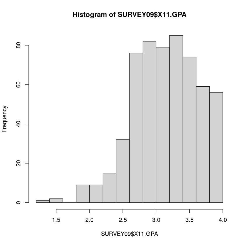
GPA could have bad values since it must be between 0 and 4 (a 0 would be a suspect value). The \(summary\) and \(hist\) look ok.
summary(SURVEY09$X11.GPA)
hist(SURVEY09$X11.GPA)
   Min. 1st Qu.  Median    Mean 3rd Qu.    Max.
  1.250   2.815   3.200   3.172   3.525   4.000
For the self-reported age at which you hope to be married, the values of 1, 2, and 4 are clearly nonsensical. Maybe they chose to answer ``How many years have you been married?’’ if they were already married.
class(SURVEY09$X22.MarriedAt)
table(SURVEY09$X22.MarriedAt)
boxplot(SURVEY09$X22.MarriedAt,horizontal=TRUE)
  1   2   4  20  21  22  23  24  25  26  27  28  29  30  31  32  33  34  35  40
  8   5   1   3   8  16  29  60 139  79  69  58   9  55   1   2   2   1  10   2
 43
  1

Note
Categorical variables: A categorical variable has possible values called levels. Possible issues:
Misspellings: e.g.
large" vs.lrge”, etc.Inconsistent Capitalization: e.g.
Male" vs.male”Inconsistent notation: e.g.
Male" vs.m” vs. ``MALE”Missing value representation: could be encoded as a blank space, numerous blank spaces, a tab, or even an NA
Redundant levels from any of the four issues above.
Making a frequency table with \(table\) or checking what unique values exist with \(levels\) can help spot errors. Note that \(summary\) also reveals how many NA’s exist (something that \(table\) cannot do).
Example: STAT 201 survey (categorical)#
Students were asked whether they voted for Obama in the 2008 election
summary(SURVEY09$X43.Obama)
levels(SURVEY09$X43.Obama)
- No
- 257
- NotVote
- 168
- Yes
- 154
- 'No'
- 'NotVote'
- 'Yes'
Do we want 3 different levels here (yes, no-voted someone else, no-did not vote at all)? Or would a yes/no suffice?
Example: DONOR database (categorical)#
Donor’s gender has an unusual value: What is “A”? Presumably “U” is unknown.
data(DONOR)
table(DONOR$DONOR_GENDER)
    A     F     M     U
    1 10401  7953  1017
Cluster Code has an unusual value: What does a “space period” represent? Is that missing?
levels(DONOR$CLUSTER_CODE)
- ' .'
- '01'
- '02'
- '03'
- '04'
- '05'
- '06'
- '07'
- '08'
- '09'
- '10'
- '11'
- '12'
- '13'
- '14'
- '15'
- '16'
- '17'
- '18'
- '19'
- '20'
- '21'
- '22'
- '23'
- '24'
- '25'
- '26'
- '27'
- '28'
- '29'
- '30'
- '31'
- '32'
- '33'
- '34'
- '35'
- '36'
- '37'
- '38'
- '39'
- '40'
- '41'
- '42'
- '43'
- '44'
- '45'
- '46'
- '47'
- '48'
- '49'
- '50'
- '51'
- '52'
- '53'
Correcting Errors#
Some errors are easy fixes: correct misspellings, combine levels that are obviously the same, remove levels. Judgment calls must be made on others (what do we do with a value of 4 for age of marriage, or a weight of 2?).
Note
Often, business domain knowledge is necessary to decide what to do with errors. Without understanding of the data and where it comes from, it can be difficult to discern the right course of action when correcting an error. This is one drawback of kaggle competitions. Most of the time variables are anonymized, so it is impossible to know what to do with suspect values.
Replacing Errors with Missing Values#
It is often good practice to replace any errors with ``missing values”, represented as an \(NA\) in R. This involves writing a sequence of commands involving \(which\) to refer to the problem elements. \(NA\) is a special symbol in R that NEVER gets double quotes (or R will treat it as a word).
Note
R encode a missing value by using the “missing value symbol” \(NA\). This \(NA\) is NEVER surrounded by quotes. If \("NA"\) is surrounded by quotes, R will treat it is the word ``NA” and not as a missing value. Be extremely careful to refer to missing values correctly.
Even though more than one element may match the condition in \(which\), it is ok to set it equal to just a single value with the left-arrow sign; it will replace all those values with NA.
#Imagine we want to turn car years less than 1950 or greater than 2010 into NA
SURVEY09$X17.CarYear[ which(SURVEY09$X17.CarYear>2010) ] <- NA
SURVEY09$X17.CarYear[ which(SURVEY09$X17.CarYear<1950) ] <- NA
#Imagine we want to take values of 1, 2, and 4 and turn them into NA
SURVEY09$X22.MarriedAt[ which(SURVEY09$X22.MarriedAt %in% c(1,2,4) ) ] <- NA
Fixing errors with categorical variables typically involves explicitly redefining the levels of the categorical variable. There is a dangerous and a safe way to do this, and refer to Unit 1 notes or Intro R Programming PDF for review.
#Make the A level of gender equal to U, since it is unknown
levels(DONOR$DONOR_GENDER)  #see the levels; redefine A to be U with the safe way
levels(DONOR$DONOR_GENDER)[ which( levels(DONOR$DONOR_GENDER) == "A" )] <- "U"
table(DONOR$DONOR_GENDER)
- 'A'
- 'F'
- 'M'
- 'U'
    U     F     M
 1018 10401  7953
Special note about \(NA\)#
When you are replacing invalid values with NA’s, be sure to refer to \(NA\) in R without any type of quotations. Putting quotes around \(NA\) makes R treat that as the word “NA” instead of treating it as a missing value.
x <- c(5,-999,12,13)
x[2] <- "NA"  #Bad bad bad, don't put NA in quotes
x  #see, it changed the vector all text
x <- c(5,-999,12,13)
x[2] <- NA  #Yes!  NA without quotes represents missingness to R
x
- '5'
- 'NA'
- '12'
- '13'
- 5
- <NA>
- 12
- 13
This is true even if we are replacing factor levels or text with NA’s!
x <- c("A","hard","to","spell","word","is","theer")
x[ which(x=="theer") ] <- "NA"  #Bad bad bad, don't put NA in quotes
x  #the last element is the WORD NA
x <- c("A","hard","to","spell","word","is","theer")
x[ which(x=="theer") ] <- NA  #Yes!  NA without quotes represents missingness to R
x
- 'A'
- 'hard'
- 'to'
- 'spell'
- 'word'
- 'is'
- 'NA'
- 'A'
- 'hard'
- 'to'
- 'spell'
- 'word'
- 'is'
- NA
Missing Data#
If a vector has missing values, then running \(mean\), \(median\), \(max\), etc., will return \(NA\) as well (since not all values are present, these quantities can’t technically be calculated).
Note
\(na.rm=TRUE\) will allow vectors with missing values.
x <- airquality$Ozone
mean(x) #returns NA because it has missing values
mean(x,na.rm=TRUE) #returns the average after missing values are excluded
max(x) #returns NA because it has missing values
max(x,na.rm=TRUE) #the maximum of the values that do exist in the data
When doing predictive analytics (fitting models), after the data values have verified (or denoted missing if invalid), you have to figure out how to treat the missing values that were generated or that have been there all along.
There is no one universally standard procedure for dealing with missing values, and many strategies have been invented over the years. They all operate on the premise that:
Note
When building a predictive model, even a relatively bad guess for a missing value is better than no guess at all.
This is because most procedures throw out from consideration any individuals who are missing just one characteristic (out of maybe hundreds recorded), which means throwing out potentially useful information.
Exploring the extent of missingness with summary#
\(summary\) on a vector or a dataframe is either a frequency table (if the variable is categorical) or the 5-number summary (if the variable is numerical). The output will also report how many missing values (which R encodes as \(NA\)) exist.
Ozone has 37 missing values while Solar.R has 7.
data(airquality)
summary(airquality)
     Ozone           Solar.R           Wind             Temp
 Min.   :  1.00   Min.   :  7.0   Min.   : 1.700   Min.   :56.00
 1st Qu.: 18.00   1st Qu.:115.8   1st Qu.: 7.400   1st Qu.:72.00
 Median : 31.50   Median :205.0   Median : 9.700   Median :79.00
 Mean   : 42.13   Mean   :185.9   Mean   : 9.958   Mean   :77.88
 3rd Qu.: 63.25   3rd Qu.:258.8   3rd Qu.:11.500   3rd Qu.:85.00
 Max.   :168.00   Max.   :334.0   Max.   :20.700   Max.   :97.00
 NA's   :37       NA's   :7
     Month            Day
 Min.   :5.000   Min.   : 1.0
 1st Qu.:6.000   1st Qu.: 8.0
 Median :7.000   Median :16.0
 Mean   :6.993   Mean   :15.8
 3rd Qu.:8.000   3rd Qu.:23.0
 Max.   :9.000   Max.   :31.0
Using \(complete.cases\) to explore missingness#
\(complete.cases()\) applied to a vector / dataframe will return a vector of \(TRUE\) or \(FALSE\) depending on if the element of that vector / row of that dataframe has all value(s) present. This output is useful for determining the extent of missingness or to easily extract all non-missing elements.
#Top four rows are complete, next two have missing values
head(airquality)
#TRUE if row is complete, FALSE if has at least one missing value
head(complete.cases(airquality))
#AIR is all rows of airquality with complete info
AIR <- airquality[ complete.cases(airquality), ]
| Ozone | Solar.R | Wind | Temp | Month | Day | |
|---|---|---|---|---|---|---|
| <int> | <int> | <dbl> | <int> | <int> | <int> | |
| 1 | 41 | 190 | 7.4 | 67 | 5 | 1 |
| 2 | 36 | 118 | 8.0 | 72 | 5 | 2 |
| 3 | 12 | 149 | 12.6 | 74 | 5 | 3 |
| 4 | 18 | 313 | 11.5 | 62 | 5 | 4 |
| 5 | NA | NA | 14.3 | 56 | 5 | 5 |
| 6 | 28 | NA | 14.9 | 66 | 5 | 6 |
- TRUE
- TRUE
- TRUE
- TRUE
- FALSE
- FALSE
Key Assumption - Missing at Random#
For most missing data imputation (replacing missing values with a good ``guess”) techniques to work, the data values must be missing at random.
Note
``Missing At Random” means that, given the other information in the data, the probability that a given value is missing does not depend on the value itself (i.e., large values are no more likely to be missing than small values).
However, it is ok for the probability of being missing to depend on other measured quantities in the data. When the missing value can be predicted from the individual’s values that do exist, imputation procedures work very well! When it cannot, replacing missing values with the median (or a new level called Missing) is easy to do.
Note
Not all missing values should be imputed!
Transformations#
Logarithmic Transformation#
Many quantities in business analytics (incomes, purchase totals, etc.), have a ``long right-hand tail”, meaning that the distribution is skewed towards larger values.
Many statistical and data mining techniques work best when the distributions of variables are as symmetric as possible. Very often, working with the logarithms of the values instead of the ones recorded is preferable.
I prefer doing log base 10, so that a 2 represents 100, 3 represents 1000, 4 represents 10000, a -2 represents 0.01, a 3.4 represents something between 1000 and 10000, etc.
In the \(DONOR\) dataset in \(regclass\), the \(Donation.Amount\) of various donors is recorded. It is very skewed right. In this case, we replace the original values with their logarithms, making the distribution much ``nicer”.
par(mfrow=c(1,2))
data(DONOR)
hist(DONOR$Donation.Amount)
DONOR$Donation.Amount <- log10(DONOR$Donation.Amount) #Overwrite values with logs
hist(DONOR$Donation.Amount)

Consider logarithmic transformations when
Dealing with quantities whose values span numerous orders of magnitudes (powers of 10)
The histogram is strongly skewed towards high values and there are extremely large outliers
Note: you can only do the logarithmic transformation if all values are LARGER than 0. Sometimes a useful trick is make numbers this way by adding a constant (often to make the smallest value equal to 1). For example, if the smallest value is -17, then add 18 to all numbers then take the log.
When doing descriptive analytics (talking about distributions and relationships) the trick of adding a constant to each value in the data to make them larger than 0 is generally ok as long as the range of original values is very large compared to the number you add (e.g., adding 18 is fine if numbers range from -17 to 10000 or more, but I wouldn’t do it if the values ranged between -17 and 3). In my opinion, it’s ok as long as it doesn’t change the magnitude or meaning of the values ``too much”.
When doing predictive analytics (building models to predict something), this trick is always ok to implement. It may or may not improve the performance of the predictive model, but it can be worth a shot.
Unlogging#
Since a lot of analytics takes place on a logarithmic scale, it’s imperative to know how to get back to the original numbers. For example, if we find the average (on the log scale) is 5.323, what ``real” value does that correspond to.
Note
To ``un-log” a value \(x\), calculate \(10^x\) (if the log base 10 had been used) or calculate \(e^x\) (if the natural log was used). If a constant \(x\) had been added to each value before logging, instead calculate \(10^x - c\), etc.
So a 5.323 corresponds to a \(10^{5.323} = 210377.8\). If 23.5 had been added to each value before logging, a 5.323 would correspond to a \(10^{5.323} -23.5 = 210354.3\)
Scaling (aka Standardizing)#
Many algorithms (particularly anything dealing with “distances” between individuals) work best when each variable is on the same “scale” (e.g., they all vary from roughly -3 to 3 instead of one ranging from 0 to a million and another ranging from 0.01 - 0.03).
The standard way of scaling a set of numbers is to subtract the average of the set of numbers from each number, then divide them by the standard deviation of the set of numbers. The new values have an average of 0 and a standard deviation of 1.
Note
Less common is scaling so that each variable ranges between 0 and 1. The \(scales\) package and \(rescale\) command can accomplish this feat if you do not wish to code it yourself, but it’s trivial to do. To scale a set of numbers, find the maximum and minimum values. Then,
Note
If all columns of a dataframe are numeric, then \(scale\) can scale dataframe in its entirety. However, the \(scale\) function outputs a matrix rather than a dataframe, so it must be ``coerced” back into a dataframe with \(as.data.frame\). If there are categorical variables, they must be omitted from \(scale\).
#dataframe whose variables are all numerical so can use scale immediately
data(EX3.ABALONE)
AB.SCALED <- as.data.frame( scale(EX3.ABALONE) )
data(CUSTCHURN)#mix of numerical and categorical columns
column.classes <- unlist(lapply(CUSTCHURN,FUN=class))#Get classes of each column
#Positions of numerical volumns
numeric.columns <- which(column.classes %in% c("numeric","integer"))
CUSTCHURN[,numeric.columns] <- as.data.frame( scale(CUSTCHURN[,numeric.columns]) )
Dates#
Many datasets have a date field to indicate when that observation was recorded. Dealing with dates can be extremely challenging regardless of what software you use to analyze data because of the myriad different formats to store this information.
Sales of each product on each date
Closing price of stocks at the end of the day
Date that new product was launched
R treats dates as a separate data type: \(POSIXct\) and \(POSIXlt\) classes. The \(as.Date\) function can be used.
See a useful writeup at: https://www.stat.berkeley.edu/~s133/dates.html
Lubridate#
library(lubridate) #load in the library every time you want to use it
Show code cell output
Attaching package: ‘lubridate’
The following objects are masked from ‘package:base’:

    date, intersect, setdiff, union
A nice tutorial can be found at: https://www.r-statistics.com/2012/03/do-more-with-dates-and-times-in-r-with-lubridate-1-1-0/
A full description from the authors is at: https://www.jstatsoft.org/article/view/v040i03/v40i03.pdf
The \(lubridate\) package does many more things:
Measure the length of time between two dates (time intervals)
Date arithmetic - rounding to the nearest month, adding 14 days to a date, etc.
Manipulation - convert a day into seconds, into fractions of a month, etc.
Please try:
To illustrate the package let us examine a data file about animals put into a shelter in Austin. The shelter data has a column called \(DateTime\) which has the time when the animal left the shelter. Since R doesn’t ``know” what is and is not a date object when reading in data, R treats this column as a categorical variable (factor).
PETS <- read.csv("shelter.csv")
class(PETS$DateTime)
head(PETS$DateTime)
- '2014-02-12 18:22:00'
- '2013-10-13 12:44:00'
- '2015-01-31 12:28:00'
- '2014-07-11 19:09:00'
- '2013-11-15 12:52:00'
- '2014-04-25 13:04:00'
To convert into dates, the first task is to figure out the date format, i.e., the ordering of the temporal information.
Date Formats#
In general, a date will contain one or more pieces of information about the year, month, day of month, hour, minute, second, and time zone. The ordering of these pieces of information will vary from source to source. To determine the ordering, simply use \(head()\) on the column of dates to take a look at the first few entries.
Looking at the first few entries of the dates in the shelter data, we see its format is YMDHMS (year/month/day/hour/minute/second). The time zone is not specified, but it is in Austin Texas. It is unclear whether or not times have Daylight Savings built in or not, but \(lubridate\) has options to handle this if it is required.
Once you have figured out what temporal information is present and its order, you are ready to use the \(lubridate\) package!
Representing Dates in lubridate#
Let us add a new column called \(Date\), which is the temporal information represented as an actual date object. Because the date was in YMDHMS format, the \(ymd\_hms\) function will be used for conversion. The function outputs an object with classes \(POSIXct\) and \(POSIXt\), which are R’s ways of storing dates!
PETS$Date <- ymd_hms(PETS$DateTime)
class(PETS$Date)
- 'POSIXct'
- 'POSIXt'
See \(?ymd\_hms\) for other conversion functions (e.g. \(dmy\_hms\)). Pretty much every way of representing dates is covered by some function!
Other formats#
How do you know which function to use in order to convert time information into a date object? Simply pay attention to how the dates are formatted and you can figure out the function easily!
``2012-09-24’’: \(ymd()\)
``09-24-2012 23:12:33’’: \(mdy\_hms()\)
``24-09-2012 10:05’’: \(dmy\_hm()\)
``2012-24-09 9’’: \(ydm\_h()\)
Power of lubridate#
The format of the dates do not have to be ``pretty” at all. \(lubridate\)’s functions are so advanced that they can usually figure out the date, even when it’s buried in with other text and written with bizarre separators. As long as you can identify the ordering of the information, you are in business!
#Let's create bizarrely formatted dates but each having
#year/month/day hour/minute/second order
x <- c(20100101120101, "2009-01-02 12-01-02", "2009.01.03 12:01:03",
       "2009-1-4 12-1-4",
       "2009-1, 5 12:1, 5",
       "200901-08 1201-08",
       "2009 arbitrary 1 non-decimal 6 chars 12 in between 1 !!! 6",
       "OR collapsed formats: 20090107 120107 (as long as prefixed with zeros)",
       "Automatic wday, Thu, detection, 10-01-10 10:01:10 and p format: AM",
       "Created on 10-01-11 at 10:01:11 PM")
ymd_hms(x)
 [1] "2010-01-01 12:01:01 UTC" "2009-01-02 12:01:02 UTC"
 [3] "2009-01-03 12:01:03 UTC" "2009-01-04 12:01:04 UTC"
 [5] "2009-01-05 12:01:05 UTC" "2009-01-08 12:01:08 UTC"
 [7] "2009-01-06 12:01:06 UTC" "2009-01-07 12:01:07 UTC"
 [9] "2010-01-10 10:01:10 UTC" "2010-01-11 22:01:11 UTC"
It’s amazing that this type of functionality and flexibility is free within R!
Extracting date information#
How do sales of a product vary from month to month, week to week, or day to day? Once the date is in the appropriate format, extracting specific information about the date is easy with the \(hour\), \(wday\), etc., commands.
just.hour <- hour(PETS$Date)
just.minute <- minute(PETS$Date)
just.day <- day(PETS$Date)
just.dayofweek <- wday( PETS$Date )  #Numbered 1, 2, 3
just.dayofweek2 <- wday( PETS$Date ,label=TRUE) #Monday, Tuesday, etc.
just.month <- month(PETS$Date)  #Numbered 1, 2, 3
just.month2 <- month(PETS$Date,label=TRUE) #January, February, etc.
just.week <- week(PETS$Date)
just.hour[1]
just.dayofweek[1]; just.dayofweek2[1]
just.month[1]; just.month2[1]
Levels:
- 'Sun'
- 'Mon'
- 'Tue'
- 'Wed'
- 'Thu'
- 'Fri'
- 'Sat'
Levels:
- 'Jan'
- 'Feb'
- 'Mar'
- 'Apr'
- 'May'
- 'Jun'
- 'Jul'
- 'Aug'
- 'Sep'
- 'Oct'
- 'Nov'
- 'Dec'
Let’s put all the exacted information we created on the previous slide into a dataframe to see more specifically what each function does.
Extraction date information
EXAMPLE <- data.frame(original=PETS$Date,hour=just.hour,minute=just.minute,
                      day=just.day,dayofweek=just.dayofweek,
                      dayofweek2=just.dayofweek2,month=just.month,
                      month2=just.month2,week=just.week)
head(EXAMPLE)
| original | hour | minute | day | dayofweek | dayofweek2 | month | month2 | week | |
|---|---|---|---|---|---|---|---|---|---|
| <dttm> | <int> | <int> | <int> | <dbl> | <ord> | <dbl> | <ord> | <dbl> | |
| 1 | 2014-02-12 18:22:00 | 18 | 22 | 12 | 4 | Wed | 2 | Feb | 7 |
| 2 | 2013-10-13 12:44:00 | 12 | 44 | 13 | 1 | Sun | 10 | Oct | 41 |
| 3 | 2015-01-31 12:28:00 | 12 | 28 | 31 | 7 | Sat | 1 | Jan | 5 |
| 4 | 2014-07-11 19:09:00 | 19 | 9 | 11 | 6 | Fri | 7 | Jul | 28 |
| 5 | 2013-11-15 12:52:00 | 12 | 52 | 15 | 6 | Fri | 11 | Nov | 46 |
| 6 | 2014-04-25 13:04:00 | 13 | 4 | 25 | 6 | Fri | 4 | Apr | 17 |
Visualization and Description#
Now we can use the date information in any analysis. For example, how does the number of adoptions/transfer/etc. vary versus day of the week?
#how many times does each day of week appear in data?
table(wday( PETS$Date,label=TRUE))
barplot( table(wday( PETS$Date ,label=TRUE)) )
 Sun  Mon  Tue  Wed  Thu  Fri  Sat
3492 2990 3177 2850 2778 2931 3511

The \(summary\) command can tell you the earliest/latest/average dates (\(min\) and \(max\) work here too). The combination of the \(names\), \(sort\), and \(table\) commands are nice to quickly see the most common/least common date components.
#how many times does each day of week appear in data?
summary(PETS$Date)
#most common to least common
sort( table(wday( PETS$Date ,label=TRUE) ), decreasing=TRUE )
#least common to most common (5 least common hours)
names( sort(table(hour( PETS$Date ))) )[1:5]
                 Min.               1st Qu.                Median
"2013-10-01 10:39:00" "2014-05-30 18:47:00" "2014-12-11 17:42:00"
                 Mean               3rd Qu.                  Max.
"2014-12-17 17:04:54" "2015-07-19 11:54:00" "2016-02-21 19:17:00"
 Sat  Sun  Tue  Mon  Fri  Wed  Thu
3511 3492 3177 2990 2931 2850 2778
- '5'
- '22'
- '6'
- '23'
- '21'