Regression (Supervised Learning)

We will start our Supervised Learning with Regression and \(tidymodels\).

library(tidymodels)
library(vip)
library(regclass)
data(LAUNCH)
data(MOVIE)
data(BODYFAT)
data(CENSUS)

Show code cell output Hide code cell output

── Attaching packages ────────────────────────────────────────────────────────────────────────────────────────────────────────────────────────────────────────────────────────────────────────── tidymodels 1.3.0 ──

✔ broom        1.0.7     ✔ recipes      1.1.1
✔ dials        1.4.0     ✔ rsample      1.2.1
✔ dplyr        1.1.4     ✔ tibble       3.2.1
✔ ggplot2      3.5.1     ✔ tidyr        1.3.1
✔ infer        1.0.7     ✔ tune         1.3.0
✔ modeldata    1.4.0     ✔ workflows    1.2.0
✔ parsnip      1.3.0     ✔ workflowsets 1.1.0
✔ purrr        1.0.4     ✔ yardstick    1.3.2

── Conflicts ───────────────────────────────────────────────────────────────────────────────────────────────────────────────────────────────────────────────────────────────────────────── tidymodels_conflicts() ──
✖ purrr::%||%()    masks base::%||%()
✖ purrr::discard() masks scales::discard()
✖ dplyr::filter()  masks stats::filter()
✖ dplyr::lag()     masks stats::lag()
✖ recipes::step()  masks stats::step()

Attaching package: ‘vip’

The following object is masked from ‘package:utils’:

    vi

Loading required package: bestglm

Loading required package: leaps

Loading required package: VGAM

Loading required package: stats4

Loading required package: splines

Attaching package: ‘VGAM’

The following object is masked from ‘package:workflows’:

    update_formula

Loading required package: rpart

Attaching package: ‘rpart’

The following object is masked from ‘package:dials’:

    prune

Loading required package: randomForest

randomForest 4.7-1.2

Type rfNews() to see new features/changes/bug fixes.

Attaching package: ‘randomForest’

The following object is masked from ‘package:ggplot2’:

    margin

The following object is masked from ‘package:dplyr’:

    combine

Important regclass change from 1.3:
All functions that had a . in the name now have an _
all.correlations -> all_correlations, cor.demo -> cor_demo, etc.

Regression Metrics

Regression models are evaluated with the following metrics:

• RMSE: the “root mean squared error”. This is the typical size of an error made by a regression model. If the estimated generalization RMSE of a model for lifetime value is $411, then this means that as-yet-unseen individuals’ actual donation amounts will be “off” from what the models predicts by $411 or so. Smaller is better, but the values depend on the units of \(y\)); its value can be sensitive to a few really bad predictions.

\[RMSE = \sqrt{ \frac{ \textrm{Sum of Squared Errors on Holdout} }{\textrm{# Observations in Holdout}} }\]

• \(\mathbf{R^2}\): the “R-squared”. A percent (0-100, or 0-1 as a decimal) that tells us how much of the observed variation in individuals’ \(y\)-values can be produced by the model. My very loose interpretation: in some sense, the model “gets you” \(R^2\) of the way there to knowing an individuals value of \(y\). If the estimated generalization \(R^2\) of the lifetime value model is 0.69, then the model will “get you” 69% of the way there” to knowing an individual’s \(y\) value.

• MAE: mean absolute error. Another measure for the typical size of an error made by the model. It’s the average of the absolute values of the errors. Its value is less sensitive to a few really bad predictions than RMSE.

\[MAE = \frac{ \textrm{Sum of Absolute Values of Errors on Holdout} }{\textrm{# Observations in Holdout}} \]

Again, it is not these values on the training that interest us, but rather what they will be on new individuals (the generalization error). We will estimate generalization errors with \(K\)-fold crossvalidation, then find the actual generalization error on our particular holdout sample to make sure it “generalizes well”.

Naive Model - worst case baseline model

The naive model takes the viewpoint that none of the predictors variables (the \(x\)’s) contain any information about \(y\).

Note

Naive Model: The predicted value of \(y\) for all individuals (in the training, holdout, or otherwise) is simply the average value of \(y\) observed in the training data for every individual. If your model cannot achieve a lower RMSE than the naive model, it is worth than using nothing to make a prediction!

The naive model is easy: Find average value of \(y\) on training data, then use it as the predicted value for all individuals.

set.seed(474)
tt_split <- initial_split(LAUNCH, prop = 0.7)
TRAIN <- training(tt_split)
HOLDOUT <- testing(tt_split)
naive <- mean(TRAIN$Profit)
POST <- HOLDOUT %>%
    select(Profit) %>%
    mutate(.pred = naive)
metrics(POST, truth = 'Profit', estimate = '.pred')

Warning message:
“A correlation computation is required, but `estimate` is constant and has 0 standard deviation, resulting in a divide by 0 error. `NA` will be returned.”

A tibble: 3 × 3

.metric	.estimator	.estimate
<chr>	<chr>	<dbl>
rmse	standard	0.4836719
rsq	standard	NA
mae	standard	0.3842963

Linear Regression Model

What you need to know:

• How linear regression models relationships (a weighted sum of some predictor variables).

• When linear regression should work well (relationships between \(y\) and each \(x\) are linear, though \(x\) can be something like \(Income^2\))

• Interpret the coefficient of a predictor variable in the output of a model (numerical and categorical)

The linear regression model essentially takes \(y\) to be a weighted sum of the predictor variables (\(x\)’s).

\[y = b_0 + b_1 x_1 + b_2 x_2 + \ldots + b_k x_k\]

• \(x_1, \ldots, x_k\) are the \(k\) features (characteristics, predictor variables, whatever you want to call them).

• The \(b\)’s of the model are the “coefficients” and represent the weights in the weighted sum.

• The \(x\) predictor variables can be the measured characteristics of an individual, e.g,. height, income, IQ, etc. or they may be transformations (\(\log Height\), \(\sqrt{IQ}\)) or even more complicated functions (\(Height/Weight^2\)).

• Predictors can be indicator variables defined to represent a categorical variable.

Note

• Linear Regression is rarely the most powerful thing you can do in predictive analytics.

• Linear Regression is a fantastic model for describing relatively simple relationships yet too simplistic for capturing intricate subtleties and squeezing out the very last bit of predictive power in the data.

• All model are wrong. Some are useful.

The real world is more complex than the linear regression model. When the regression model provides a reasonable reflection of reality, it’s a great tool for talking about what relationships look like. However, the regression model typically misses out on subtleties (not important for the general discussion of what relationships look like) that makes it a relatively poor choice for making predictions.

In predictive analytics, we don’t require the model to provide a reasonable description of reality as long as it’s making accurate predictions (of course, a model that does describe reality well should predict well too). The simple linear regression below does not provide a realistic description of the relationship, but it’s predictions come “pretty close”.

x<-runif(100, 2, 10); y<-3*x^2; plot(y~x,pch=20);abline(lsfit(x,y),col="red",lwd=3)

Interpretation

Model: Predict the tip percentage left on a bill based on the amount of the bill (numerical), gender of the paying party (categorical), smoking section (categorical), day of week (categorical), and time of day (categorical).

                Estimate Std. Error t value Pr(>|t|)  
(Intercept)     20.19552    2.36514   8.539 1.71e-15 ***  <-- b0
Bill            -0.28225    0.05393  -5.234 3.68e-07 ***  <-- "Estimate" is coefficient (b) 
GenderMale      -0.45700    0.79538  -0.575    0.566    
SmokerYes        1.24699    0.82333   1.515    0.131    
WeekdaySaturday -0.31426    1.73971  -0.181    0.857  <--- Indicator variable = 1 if Saturday 0 Otherwise 
WeekdaySunday    1.45871    1.80461   0.808    0.420    
WeekdayThursday -0.73705    2.20962  -0.334    0.739    
TimeNight       -0.67806    2.49725  -0.272    0.786  <--- Indicator variable = 1 if Night 0 Otherwise 

Residual standard error: 5.753 on 235 degrees of freedom
Multiple R-squared:  0.1421,	Adjusted R-squared:  0.1129 
F-statistic: 4.866 on 8 and 235 DF,  p-value: 1.438e-05

Interpretation of Numerical Predictor

Model: Predict the tip percentage left on a bill based on the amount of the bill (numerical), gender of the paying party (categorical), day of week (categorical), and time of day (categorical).

                Estimate Std. Error t value Pr(>|t|)  
Bill            -0.28225    0.05393  -5.234 3.68e-07 ***  <-- "Estimate" is coefficient (b) 

Two “otherwise identical individuals” (in regards to the other predictors in the model) who differ in \(x\) by one unit are expected to differ in \(y\) by \(b\) units.

Two otherwise identical bills (paid by same gender, in the same type of smoking/nonsmoking section, on the same day and time of day) that differ in amount by $1 are expected to differ in tip percentage by 0.28%, with the larger bill expected to be lower (since the coefficient is negative).

Interpretation of Categorical Predictor

Each level of a categorical variable (except the first alphabetically, which serves as a reference) gets its own indicator variable to represent it in the model (R will take the name of the column and append the name of the level to come up with the name of the indicator variable)

                Estimate Std. Error t value Pr(>|t|)  
SmokerYes        1.24699    0.82333   1.515    0.131  <--- Indicator variable = 1 if Yes 0 No

The difference in the average value of \(y\) (among “otherwise identical individuals” with respect to the predictors in the model) between individuals with the featured level vs. individuals with the reference level is \(b\).

The difference in the average tip percentage (on bills that are the same amount and are paid by the same gender, on the same day and time of day) between smokers and nonsmokers is 1.2% (with smokers being higher since the coefficient is positive and “No” is the reference level).

                Estimate Std. Error t value Pr(>|t|)  
WeekdaySaturday -0.31426    1.73971  -0.181    0.857  <--- Indicator variable = 1 if Saturday 0 Otherwise 
WeekdaySunday    1.45871    1.80461   0.808    0.420    
WeekdayThursday -0.73705    2.20962  -0.334    0.739    

The difference in the average value of \(y\) (among “otherwise identical individuals” with respect to the predictors in the model) between individuals with the featured level vs. individuals with the reference level is \(b\).

The difference in the average tip percentage (on bills that are the same amount and are paid by the same gender, in the same type of smoking/nonsmoking section, and during the same time of day) between Saturdays and Fridays 0.3% (with Saturday being lower because the coefficient is negative and “Friday” is the reference level).

Key quantities of a regression read off \(summary\)

Residual standard error: 5.753 on 235 degrees of freedom
Multiple R-squared:  0.1421,	Adjusted R-squared:  0.1129 

• \(Residual Standard Error\) (RMSE / Root Mean Squared Error) - a name for the typical size of a residual, the typical error made by the regression, or the typical distance between the regression and actual points (all 3 quantities are equivalent). This is on the training data so of no immediate interest.

• \(Multiple R-Squared\) (\(R^2\)) - the model “gets you” about \(R^2\) of the way there to knowing \(y\). Used to gauge how well the model fits the data, though a high \(R^2\) does not necessarily mean the model is appropriate for describing the relationship (could be nonlinear). This is on the training data so of no immediate interest.

• \(Adjusted R-squared\) (\(R^2_{adj}\))- a fairer measure of how well the model fits the data since it incorporates a penalty based on how many \(x\)’s are in the model (an additional \(x\) always makes \(R^2\) get larger, even when \(x\) has no association with \(y\)). This is on the training data so of no immediate interest.

Interaction Between Variables

For many problems, interactions between variables often play an important role.

• If \(x_1\) and \(x_2\) have an interaction, then the form/strength of the relationship between \(y\) and \(x_1\) depends depends on the exact value of \(x_2\) under consideration (sale price of homes rise much more quickly with square area in NYC than in Knoxville, so “area” and “location” have an interaction).

• Interactions are easy to put into a regression model (use the predictor variable \(x_1 \cdot x_2\)), but knowing which interactions to put in is difficult.

When there are \(k\) predictor variables, there are \(k(k-1)/2\) possible interactions that could be included. For “small” data mining problems with \(k=8\) this is 28 predictors. For “larger” data mining problems with \(k=100\) this is 4950 predictors.

Note

In data mining, we will learn many advanced models that can automatically incorporate interations instead of manually specifying a complex linear regression.

Equation is not a physical law

Just because linear regression gives us equation to describe the relationship, the equation is NOT a physical law like \(E=mc^2\).

While equations in physics describe what happens to something when its properties change, a regression equation only tries to capture in mathematical form how the \(y\) values of various individuals are expected to differ.

The regression equation makes NO comment about what will happen to an individual’s \(y\) value when his/her \(x\) values gets larger.

Complication: transforming \(y\) and \(x\)

When predicting numerical responses (with linear regression or the more complex models we will discuss), we need to worry about what exactly is to be our \(y\) variable (the “response” we are trying to predict). For example, imagine trying to predict the weekly sales of a product that is sold on a TV shopping network.

• \(y =\) sales?

• \(y = \log_{10} (sales)\)? Perhaps, if skewed.

• \(y = \) sales/(duration \(\times\) viewers)? Since a product will sell more the longer its been shown on TV and when more people are watching, it may be useful to “normal” sales and think of it as sales per viewer per hour.

• \(y = \log_{10}\) sales/(duration \(\times\) viewers)? Perhaps, if skewed.

Note

Picking the right response to predict is imperative for predictive analytics!

Of critical importance is making sure that the \(y\) variable (whatever that turns out to be) is not “too skewed”.

• Outliers tend to exert more than their fair share of influence on the coefficients of the model. It would be “nice” if all individuals contributed more or less equal information to the model.

• If the form of a model is sensitive to the set of individuals that happen to be in the training data (as we will see when we discuss the bias/variance tradeoff), then it will potentially have large generalization error!

• When \(y\) is skewed, the model has difficulty predicting outliers. Our impression of the typical error is unduly influenced by these oddballs, which may not be fair.

Note

Making the variable we want to predict (\(y\), the response variable) symmetric through the use of transformations like logarithms, square roots, etc., almost always makes the model generalize better to new data.

The first step when making a predictive model for \(y\) is to look at the distribution of \(y\) to see if we need to transform it!

Choose the “right” \(y\) (raw recorded values, some function of quantities, etc.) is important as well but often this requires domain-specific understanding of the problem (e.g., TV sales example).

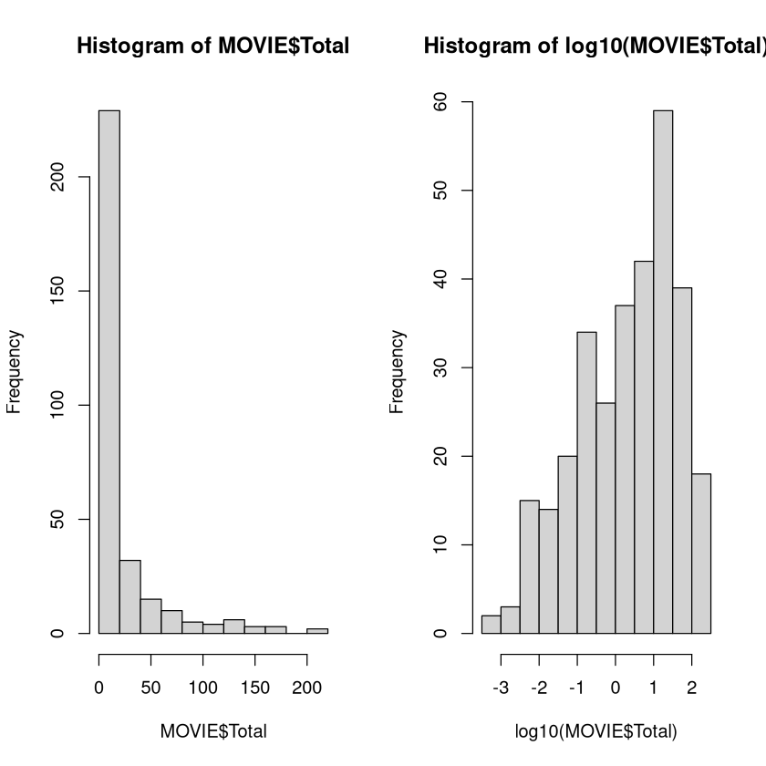
Imagine you were going to develop a model that predicted the total amount of money a movie makes. The first step is to look at the distribution of the total gross.

The histogram of the recorded values is extremely skewed. This makes it difficult for a model to make predictions (especially for higher amounts). We would want to build a model to predict the logarithm of the gross instead, which has a much more symmetric distribution.

par(mfrow=c(1,2))
hist(MOVIE$Total)
hist(log10(MOVIE$Total))

Transformations of \(x\) (Predictor Variables) is also important. Most algorithms in data mining “work better” if the distributions of the predictor variables looked roughly symmetric as well (we saw this with clustering).

• Outliers have the potential to greatly influence the coefficients and form of the model, thus making the model sensitive to a few individuals. Models whose form is very sensitive to the particular set of individuals that happen to be in the training data have a “high variance” and potentially a large generalization error.

• Regression models (both linear and logistic) tend to work better with symmetric predictors.

• Nearest Neighbors and Support Vector Machines tend to work better with symmetric predictors, though making transformations changes somewhat the notion of similarity (or “inner product”) between individuals.

• Tree-based models introduce rules between 2 unique values of predictor variables so symmetry/skewness is not relevant (the same sets of individuals will be above/below a chosen threshold regardless of whether a transformation of the predictor is made)!

Pros and Cons of Linear Regression

For predictive analytics, linear regression has a few pros but many cons.

Note

Pros:

• Easily interpretable. Once a model has been fit, it is easy to describe how it models the relationship between \(y\) and any particular predictor variable (even those involved in interactions).

• Making predictions is easy: plugging numbers into an equation.

• If assumptions hold behind a model, you can put confidence intervals on predictions (no other model we’ll talk about has this feature).

• It is really the only statistical model we will consider (meaning its theoretical properties are well known and we can talk about the accuracy of its estimates and predictions with a certain level of confidence).

Cons for using Linear Regression for Predictive Analytics:

• Form of model is chosen in fundamentally the wrong way. Coefficients of the model are chosen to minimize its bias, without regard to how well it generalizes to new data (need regularization; stay tuned).

• Interactions can be difficult to put in the model, mostly because there are often too many to consider. A regression won’t find an interaction without us explicitly putting it in the model. Since interactions are often very important, when there are a lot of variables this makes the task difficult.

• Have to choose what exactly to use as the predictor variables. The measured quantities? Their logarithms? Some other transformation? Some function of multiple variables as a predictor? Our decision matters and effects the quality of the model.

• We have to choose which predictor variables to include. With 30 predictors, there are \(2^{30}\) = 1 billion combinations of variables that could be used as predictors (if no interactions were considered; way more if they are). Variable selection can be very slow.

Despite the cons, linear regression is often an “acceptable” model (and sometimes the best), though you can usually do better.

Regularized Regression

Signal vs. Noise

We say that a characteristic that does indeed contain information about the quantity we are trying to predict is a “signal” or a “signal feature”. One that does not is referred to as “noise”. For example, when predicting your weight, your height would be a “signal” but your favorite color is (likely) “noise”.

In general, adding additional signal features that are truly associated with an individual’s value of \(y\) will improve the fitted model (reduce its generalization error).

Adding noise features that are not truly associated with an individual’s class will lead to a deterioration in the fitted model, and consequently an increased generalization error. This is because noise features increase the risk of overfitting (since they may be given nonzero coefficients due to purely chance associations with \(y\)) without any potential upside in terms of reduced generalization error.

So is more data a bad thing?

Collecting thousands or millions of characteristics to use for predictions is a double-edged sword.

They can lead to improved predictive models if these characteristics are in fact relevant to the problem at hand (signal), but will lead to worse results if they are irrelevant (noise).

However, even if they are relevant, the variance in the model-building procedure incurred in fitting their coefficients may outweigh the reduction in bias that they bring.

The problem

All models in predictive analytics have a common problem: the variance of a model is high if it uses unnecessary or irrelevant predictor variables (i.e. extracts more information than it needs, making it unduly sensitive to the individuals that happen to be in the training data).

In other words, models will be overfit (by definition) if they try to incorporate information from unrelated predictors (all models will find some patterns between \(y\) and the \(x\)’s, even if those characteristics are meaningless).

For example, imagine we fit a simple linear regression predicting \(y\) from \(x\) when, in reality, they are completely unrelated. We will never measure a slope that’s exactly zero - the model always finds some pattern (however weak).

set.seed(474)
xy <- data.frame(x = runif(20), y = runif(20))
fit(linear_reg(), y~x, data = xy)

parsnip model object


Call:
stats::lm(formula = y ~ x, data = data)

Coefficients:
(Intercept)            x  
     0.4280       0.2346  

Coefficient is pretty far from 0 even though x and y are unrelated!

The problem: how can we do feature selection (choosing which variables to include in the model) in an efficient manner so that we can avoid overfitting and avoid high variance?

• Naive Bayes, Linear/Logistic Regression, \(K\)-nearest neighbors, neural networks, and support vector machines use information from all predictors input into the model (even if those predictors contain no useful information). Unnecessary predictors tend to mask and diminish the importance of useful predictors and their inclusion decreases a model’s accuracy. Big Issue!

• Tree-based models (vanilla partition, random forest, boosted tree) automatically select the “important” variables to include in the model, so this is less than an issue.

Illustration of unnecessary predictors

In the \(BODYFAT\) data, we predict someone’s body fat percentage from their physical characteristics. modeled the probability that a cockroach would die given a particular dose of poison. The typical error on “new” data is about 4 percentage points.

set.seed(474)
tt_split <- initial_split(BODYFAT, prop = 0.6)
TRAIN <- training(tt_split)
HOLDOUT <- testing(tt_split)
MODEL <- linear_reg() %>%
    fit(BodyFat~., data = TRAIN)
POST <- HOLDOUT %>%
    select(BodyFat) %>%
    bind_cols(predict(MODEL, new_data = HOLDOUT))
metrics(POST, truth = 'BodyFat', estimate = '.pred')

A tibble: 3 × 3

.metric	.estimator	.estimate
<chr>	<chr>	<dbl>
rmse	standard	4.3393362
rsq	standard	0.7445379
mae	standard	3.5762965

Let’s look at the variable importances.

vip(MODEL)

Abdomen is “most important” predictor, followed by Wrist, Age, etc. What if we threw in a bunch of irrelevant predictors (just random numbers)? How does the model do with the added “noise”?

set.seed(474)
#Make a data frame of 20 irrelevant predictors
RANDOM <- as.data.frame( matrix( runif( 20*nrow(BODYFAT) ), ncol=20 ))
tt_split <- initial_split(cbind(BODYFAT, RANDOM), prop = 0.6)
TRAIN <- training(tt_split)
HOLDOUT <- testing(tt_split)
MODEL <- linear_reg() %>%
    fit(BodyFat~., data = TRAIN)
POST <- HOLDOUT %>%
    select(BodyFat) %>%
    bind_cols(predict(MODEL, new_data = HOLDOUT))
metrics(POST, truth = 'BodyFat', estimate = '.pred')

A tibble: 3 × 3

.metric	.estimator	.estimate
<chr>	<chr>	<dbl>
rmse	standard	5.0103319
rsq	standard	0.6507087
mae	standard	4.0905225

The addition of 20 irrelevant predictors will make the model “fit noise” in addition to the useful information contained in the dose. The relationship between bodyfat percentage and physical characteristics gets somewhat obscured by the irrelevant information, making the typical error increase from 4.3 to 5.0.

Let’s look at the variable importances.

vip(MODEL)

The model still knows that Abdomen is the most important variable, but many irrelevant predictors have creeped into the top 10.

What about adding in even more irrelevant information?

set.seed(474)
#Make a data frame of 100 irrelevant predictors
RANDOM <- as.data.frame( matrix( runif( 100*nrow(BODYFAT) ), ncol=100 ))
tt_split <- initial_split(cbind(BODYFAT, RANDOM), prop = 0.6)
TRAIN <- training(tt_split)
HOLDOUT <- testing(tt_split)
MODEL <- linear_reg() %>%
    fit(BodyFat~., data = TRAIN)
POST <- HOLDOUT %>%
    select(BodyFat) %>%
    bind_cols(predict(MODEL, new_data = HOLDOUT))
metrics(POST, truth = 'BodyFat', estimate = '.pred')

A tibble: 3 × 3

.metric	.estimator	.estimate
<chr>	<chr>	<dbl>
rmse	standard	8.1181749
rsq	standard	0.4471033
mae	standard	6.3545666

With 100 irrelevant predictors, the relationship between bodyfat percentage and physical characteristics is almost completely washed out. Let’s look at the variable importances.

vip(MODEL)

The model STILL knows that Abdomen and Knee are important variables, but the rest of the top 10 is noise!

Variable Selection via Regularization

We can address the problem of variable selection by trying out models that contained different subsets of predictors and picking one whose estimated generalization error was reasonable.

• \(regsubsets\) fit all regressions that used a single predictor, all regressions that used a pair of predictors, all regressions that used a trio of predictors, etc. Interactions may or may not be included. This “best subsets” approach is very effective but computationally very slow (especially for logistic regression).

• \(step\) performed a search for a reasonable model by augmenting a starting model in stages. At each stage, either a new variable is added to the regression or an existing one is eliminated from it (whichever move drove the model “closer to the truth”). While there is no guarantee of finding “the best” model, a “good” one is often found.

We will take the viewpoint that the subsets and search procedures for selecting the predictors to go into a regression model are way too slow. Instead, we will use regularization to (nearly) avoid the task of variable selection altogether. Regularization is a fancy term that merely means modifying what it means for the model to “best fit” the data.

• Least Squares regression: coefficients are chosen so that the resulting model has the smallest sum of squared errors possible. Coefficients in logistic regression are chosen in a different manner (maximum likelihood), but the overall idea is roughly analogous.

• Ridge regression: coefficients are chosen to balance the resulting model’s sum of squared errors and sum of squared coefficients (i.e., large coefficients incur a penalty).

• Lasso: coefficients are chosen to balance the resulting model’s sum of squared errors and sum of absolute values of coefficients (i.e., large coefficients incur a penalty, but not as large as in ridge regression).

• \(glmnet\): a combination of ridge regression and the lasso.

Multiple Linear Regression and the “Loss Function”

Given a set of features of individuals \(x_1\), \(x_2\), \(\ldots\), \(x_k\), the fitted multiple linear regression model is essentially a weighted sum of the characteristics:

\[Predicted = b_0 + b_1 x_1 + b_2 x_2 + \ldots b_k x_k\]

The values of the coefficients \(b_0\), \(b_1\), etc., are chosen via the “least squares” criteria, so that the sum of squared errors made by the resulting model is as small as possible.

\[Loss = SSE = \textrm{Sum of Squared Errors} = \textrm{Sum of } (Actual - Predicted)^2\]

People refer to the \(SSE\) as the loss function and its value is to be minimized.

Residuals

To find the line that fits the data “the best”, it makes sense to minimize the amount of error that the line makes. An error is better known as a residual is the difference between the observed (actual) value of \(y\) and the value of \(y\) predicted by the equation (i.e., the location of the line).

\[Residual \,\, (Error) = Actual - Predicted\]

Residuals can be positive (if the point is above the line) or negative (point is below the line).

set.seed(1990)
x <- 1:5
y <- round( (5 + 2*x + rnorm(5,0,5)),digits=1)
plot(x,y,pch=20,cex=2)
M <- lm(y~x)
abline(M)
lines( c(2,2), c(y[2],predict(M)[2]),lwd=3,col="red")
lines( c(3,3), c(y[3],predict(M)[3]),col="red",lwd=3)
text(2,12.78,"Residual=10.2-6.78=3.42",cex=0.6)
text(3,5.15,"Residual=7.2-9.16= -1.96",cex=0.6)

Note

By picking coefficients that minimize \(SSE\) on the training data, we are essentially minimizing the “bias” of the model while paying no attention to its resulting “variance”. This is a problem if the goal of the model is to generalize to new individuals! Thus, the form of the vanilla linear regression model is chosen in fundamentally the wrong way.

Ridge Regression

In ridge regression, the loss function is:

\[Loss = SSE + \lambda \cdot \left( b_1^2 + b_2^2 + \ldots + b_k^2\right)\]

Here, \(\lambda \ge 0\) is a “tuning” parameter that helps control the bias-variance tradeoff (the “right” value must be found via cross-validation).

• The first term in the loss is the sum of squared errors (\(SSE\)). To make the loss small, we want the SSE to be as small as possible, just like in standard regression.

• The second term is the shrinkage penalty. To make the loss small, we want the coefficients to be as close to 0 as possible (i.e. use the least amount of information that we can from the predictor variables). When \(\lambda\) grows in size, the effect is to “shrink” the coefficients closer to 0 relative to the numbers standard regression would provide.

We want our predictive model to explain the most it can about the relationships (i.e., have the smallest sum of squared errors possible) while using the least amount of information it can (i.e., have the smallest values of the coefficients).

• If predictors are scaled, then their magnitude is a measure of how much information that model uses from that predictor (values farther from zero, positive or negative, mean more information).

• The sum of squared coefficients thus provides a rough measure of how much information the model is extracting from the dataset.

• The \(Loss\) then roughly measures \(Bias^2\) (SSE) plus \(Variance\) (sum of squared coefficients), which is our equation for the MSE, the expected generalization error!

• Irrelevant predictors “should” have coefficients of 0. Ridge regression would like to make the coefficients as small as possible, so this should drive the coefficients of irrelevant predictors close to 0.

• Important predictors “should” have large coefficients (since all predictors are scaled, the size of the coefficient does roughly indicate its importance to the model). Ridge regression would like to make the coefficients as small as possible, so if a characteristic gets a large coefficient it should be truly predictive of the class labels.

• Small \(\lambda\) \(\rightarrow\) low bias (more flexibility, more information extracted from training data, and less error on training data) but potentially high variance (bad generalizability).

• Large \(\lambda\) \(\rightarrow\) high bias (less flexibility, less information extracted from training data, and more error on training data) but potentially lower variance (better generalizability).

• Should be able to find an “ideal” value of \(\lambda\) that provides a good compromise between simplicity and generalizability.

The “optimal” complexity of the model, i.e., “best” value of \(\lambda\) can be estimated via cross-validation!

Lasso Regression

The lasso uses the loss function:

\[Loss = SSE + \lambda \cdot \left( |b_1| + |b_2| + \ldots + |b_k|\right)\]

• Very similar to ridge regression, but the amount of information extracted from the training data (sum of absolute values of coefficients) is different.

• Big difference between lasso and ridge: lasso \(\lambda\) penalty can end up forcing some coefficients to be exactly zero (ridge penalty only makes them very small).

• Lasso thus does automatic variable selection! This is why the lasso is often preferred for problems with LOTS of predictors.

Note

Important note about scaling.

Because the sizes of coefficients depend on the units in which the characteristics are recorded, it is important to scale the predictors to have a mean of 0 and a standard deviation of 1 before doing ridge regression or the lasso.

This way, the size of a coefficient effectively measures how much information the model is extracting from that predictor! Further, the size penalty is also applied equally to all predictors!

glmnet

The \(glmnet\) method allows us to do regularization, including ridge regression and the lasso. In fact, it allows you to blend the two approaches together.

\[Loss = SSE + \lambda \cdot \left( 0.5(1-\alpha)(\text{Sum of $b^2$'s}) + \alpha(\text{Sum of $|b|$'s}) \right)\]

When \(\alpha=0\), it is basically ridge regression. When \(\alpha=1\) it is basically the lasso. For values of \(\alpha\) in the middle it is a blend of the two methods. When predictors are highly correlated with one another, mixing this methods is a good strategy since the lasso tends to throw out one of the correlated predictors while ridge regression tends to give them equal coefficients.

Important

Compare the below \(glmnet\) model with the \(pca\) model in the previous chapter.

set.seed(474)
tt_split <- initial_split(CENSUS, prop = 0.7)
TRAIN <- training(tt_split)
HOLDOUT <- testing(tt_split)

REC <- recipe(ResponseRate ~ ., TRAIN) %>%
    step_nzv(all_predictors()) %>%
    step_corr(all_predictors()) %>%
    step_lincomb(all_predictors()) %>%
    step_interact(terms = ~ all_predictors()^2)

WF <- workflow() %>%
    add_recipe(REC) %>%
    add_model(linear_reg( engine = 'glmnet', penalty = tune(), mixture = tune() ))

RES <- WF %>%
    tune_grid(
        resamples = vfold_cv(TRAIN, v = 5),
        grid = grid_regular(penalty(), mixture()),
    )

METRICS <- RES %>%
    collect_metrics() %>%
    select(penalty, mixture, .metric, mean, std_err)

METRICS

A tibble: 18 × 5

penalty	mixture	.metric	mean	std_err
<dbl>	<dbl>	<chr>	<dbl>	<dbl>
1e-10	0.0	rmse	4.6820504	0.096974838
1e-10	0.0	rsq	0.6085073	0.008453923
1e-05	0.0	rmse	4.6820504	0.096974838
1e-05	0.0	rsq	0.6085073	0.008453923
1e+00	0.0	rmse	4.6758570	0.106472769
1e+00	0.0	rsq	0.6086518	0.009751629
1e-10	0.5	rmse	5.0042071	0.096251269
1e-10	0.5	rsq	0.5713964	0.013432655
1e-05	0.5	rmse	5.0042071	0.096251269
1e-05	0.5	rsq	0.5713964	0.013432655
1e+00	0.5	rmse	4.8991136	0.137890279
1e+00	0.5	rsq	0.5787666	0.016089196
1e-10	1.0	rmse	5.0257588	0.095707592
1e-10	1.0	rsq	0.5689644	0.013862823
1e-05	1.0	rmse	5.0257588	0.095707592
1e-05	1.0	rsq	0.5689644	0.013862823
1e+00	1.0	rmse	5.0841433	0.135234860
1e+00	1.0	rsq	0.5627520	0.017054983

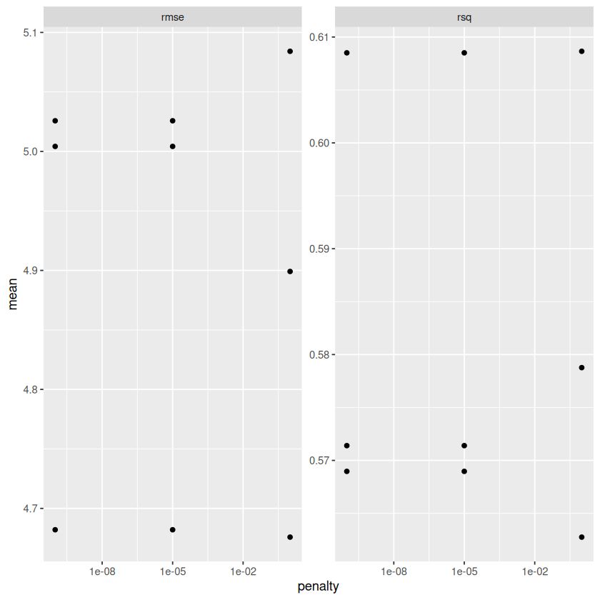
METRICS %>%
    ggplot(aes(mixture, mean)) + geom_point() + facet_wrap(~ .metric, scales = "free")

METRICS %>%
    ggplot(aes(penalty, mean)) + geom_point() + facet_wrap(~ .metric, scales = "free") + scale_x_log10()

MODEL <- WF %>%
    finalize_workflow(
        select_best(RES, metric = "rmse")
    ) %>%
    fit(
        TRAIN
    )
MODEL

══ Workflow [trained] ══════════════════════════════════════════════════════════════════════════════════════════════════════════════════════════════════════════════════════════════════════════════════════════════
Preprocessor: Recipe
Model: linear_reg()

── Preprocessor ────────────────────────────────────────────────────────────────────────────────────────────────────────────────────────────────────────────────────────────────────────────────────────────────────
4 Recipe Steps

• step_nzv()
• step_corr()
• step_lincomb()
• step_interact()

── Model ───────────────────────────────────────────────────────────────────────────────────────────────────────────────────────────────────────────────────────────────────────────────────────────────────────────

Call:  glmnet::glmnet(x = maybe_matrix(x), y = y, family = "gaussian",      alpha = ~0) 

     Df  %Dev Lambda
1   528  0.00 4936.0
2   528 12.19 4498.0
3   528 13.14 4098.0
4   528 14.15 3734.0
5   528 15.22 3402.0
6   528 16.33 3100.0
7   528 17.51 2825.0
8   528 18.73 2574.0
9   528 20.00 2345.0
10  528 21.32 2137.0
11  528 22.67 1947.0
12  528 24.07 1774.0
13  528 25.49 1616.0
14  528 26.94 1473.0
15  528 28.40 1342.0
16  528 29.88 1223.0
17  528 31.36 1114.0
18  528 32.84 1015.0
19  528 34.30  924.9
20  528 35.75  842.7
21  528 37.18  767.9
22  528 38.56  699.7
23  528 39.90  637.5
24  528 41.19  580.9
25  528 42.44  529.3
26  528 43.63  482.3
27  528 44.77  439.4
28  528 45.85  400.4
29  528 46.86  364.8
30  528 47.83  332.4
31  528 48.73  302.9
32  528 49.57  276.0
33  528 50.35  251.4
34  528 51.08  229.1
35  528 51.77  208.8
36  528 52.40  190.2
37  528 52.99  173.3
38  528 53.54  157.9
39  528 54.06  143.9
40  528 54.53  131.1
41  528 54.98  119.5
42  528 55.39  108.8
43  528 55.78   99.2
44  528 56.14   90.4
45  528 56.48   82.3
46  528 56.81   75.0

...
and 54 more lines.

vip(MODEL)

POST <- HOLDOUT %>%
    select(ResponseRate) %>%
    bind_cols(predict(MODEL, new_data = HOLDOUT))
metrics(POST, truth = 'ResponseRate', estimate = '.pred')

A tibble: 3 × 3

.metric	.estimator	.estimate
<chr>	<chr>	<dbl>
rmse	standard	4.9914402
rsq	standard	0.5667216
mae	standard	3.5885099

Review: Regularization

We will see that most model-building procedures have the fundamental flaw that its form (coefficients of predictors, rules, etc.) is chosen to minimize the model’s bias while ignoring its variance entirely.

• Coefficients in logistic regression were chosen to make the resulting model have the highest chance of reproducing the training data (smallest bias).

• Rules are added in a partition tree to minimize the resulting partitions’ impurity (smallest bias).

The form of a model should be chosen by considering both its bias and its variance. This is what regularization accomplishes.

Regularizing a model makes it so that its form is explicitly influenced by both the model’s bias and variance.

• Ridge regression and the lasso chose its coefficients so that the resulting model minimized a weighted sum between the error it made and its complexity (measured in terms of the sizes of coefficients).

• XGBoost chooses the form of each tree by penalizing its size and regularizing how the decrease in impurity is calculated via the \(gamma\) and \(lambda\) parameters. \url{http://xgboost.readthedocs.io/en/latest/model.html}

Most models for predicting numerical responses still suffer from the flaw that the form of the model is chosen to minimize the model’s bias while paying no attention to the model’s variance.

We compensate somewhat by fitting many versions of that model (different tuning parameters), estimating the generalization errors of each, and choosing one with the lowest. However, it would be nice if the model’s generalization was built-in to the procedure for estimating its form!

In predictive analytics, our goal is a model that explains as much as possible about the relationships observed among individuals while using the least amount of information in the data that we can get away with (getting the “gist” of the relationship usually yields the best generalization).

Minimizing the loss function allows us to do just that!

• Explaining as much as possible about the relationships means making the SSE as small as possible.

• Using as little information possible means making the coefficients as small as possible.

• Somewhere, there is a good balance between the extent of the relationships we are modeling and the amount of information we are using to give the best generalization possible!

Pros and Cons of regularization:

Note

Pros:

• “Fixes” a fundamental problem with “vanilla” linear and logistic models (choosing the coefficients so they specifically have the generalization error of that model in mind).

• Lasso allows automatic feature selection by setting some coefficients exactly to 0.

• Mathematically shown that regularizing always gives a better model (a value of \(\lambda=0\) gives vanilla regression anyway, so it’s just a special case of the models being fit).

Cons:

• A bit more pre-processing of data has to be done (scaling the predictors)

• Even though this “fixes” linear/logistic regression, it’s still rarely the best predictive model out there.